Recap of Fundamentals in Aerodynamics - 2D and 3D
Contents
Recap of Fundamentals in Aerodynamics - 2D and 3D
… if we all designed bodies to have stagnation points at the back, then D’Alembert would rest happy, and we would have no drag. Presumably that would be a Good Thing generally, except for parachutists!
It’s easy to explain how a rocket works, but explaining how a wing works takes a rocket scientist.
Aerodynamic theory is now (1930) rather like the physical theory of light; Sir William Bragg recently said that physicists use the electron theory on Mondays, Wednesdays and Fridays, and the wave theory on alternate days. Both have uses but reconciliation of the two ideas has not yet been achieved. So it is in aeronautics. In our experimental work we assume that viscosity is an essential property of air and the building of a compressed-air tunnel is the latest expression of that belief. The practically useful theory of Prandtl comes from considering air as frictionless or inviscid.
To those who fear flying, it is probably disconcerting that physicists and aeronautical engineers still passionately debate the fundamental issue underlying this endeavor: what keeps planes in the air?
STAYING ALOFT; What Does Keep Them Up There?
On a strictly mathematical level, engineers know how to design planes that will stay aloft. But equations don’t explain why aerodynamic lift occurs. There are two competing theories that illuminate the forces and factors of lift. Both are incomplete explanations. Aerodynamicists have recently tried to close the gaps in understanding. Still, no consensus exists.
This chapter is a whirlwind tour of some of the basics of airfoil aerodynamics that is relevant for this course. Since airfoils can be imagined as the basic building blocks that make up the rotor, the fundamental understanding of airfoil aerodynamics laid down here would help develop a more intuitive understanding of rotor aerodynamics. As some of the quotes above imply, the mathematical theory of fluid behavior, and by extension the mathematiacl theory of flight, are well established. However, given the complex equations involved a straightforward cause and effect relation is difficult to establish and hence a simple intuitive explanation for something even as common and fundamental as the process of lift generation on an airfoil is still missing. Nevertheless, below we try to make as much progress as possible in the improving/refreshing the understanding of the fundamental fluid dynamics concepts involved. It is hoped that the discussions in this chapter will make the fundamental concepts, underlying much of fluid dynamics, more intuitive than the involved mathematical equations themselves.
This chapter is predominantly based on the content in [McL13], in particular Chapter 7 from this reference. Additionally, [PJ06a] and [PJ06b] provide a good overview of the historical development of the field of fluid dynamics.
Bodies in fluids
Understanding the nature of forces acting on bodies of arbitrary shape is in our interest if the objective is to minimise the amount of work done in order to overcome the resistive forces due to friction caused due to relative motion between the body and the surrounding fluid. Optimum hull design of a cruise ship, minimum drag profile of a competitive road cyclist+cycle etc are a few examples where an understanding of fluid behavior would help achieve the objectives. Of course, we need not look too far for examples because a helicopter has various entities that might benefit from design based on a sound knowhow in fluid dynamics. A streamlined fuselage design such that drag (rotorcraft fuselage drag is referred to as parasite drag) is minimised would go a long way in reducing operating costs.
Some fundamental laws are followed by real fluids -
conservation laws
energy, linear momentum and mass
they cannot penetrate the body surface (\(F\))
Fluid cannot penetrate the surface of the body in consideration. This seems like a trivial concept to state explicitly but remember that when a problem involving fluids is mathematically stated, the condition at the boundaries of the fluid need to be clearly defined. In the case of an airfoil moving about in infinite fluid, the surface of the airfoil forms one of the boundaries (the other boundary is at infinite distance away and not a source of any disturbance). What happens to the fluid at this boundary, i.e. the surface of the airfoil, dictates what happens in the rest of the fluid. This behavior of the fluid, specifically the velocity in the case of an incompressible flow, is the quantity of interest because this would then eventually lead to the amount of lift generated from the subsequent behavior of the fluid due to the airfoil motion. Since we know from physical observations that fluid parcels do not permeate through object surfaces, the motion of the fluid at this boundary is exactly matched with the motion of the airfoil surface. This is refered to as the no penetration boundary condition.
Any model of (Newtonian) fluids would have to satisfy the above laws and we do have a model that does that - the Navier-Stokes equations.
Navier-Stokes equations (NSE)
The NSE are essential to so many analyses you encounter involving fluid flows yet they can be solved without the use of a computer for only a handful of idealised scenarios. Even today, the fact that these equations are challenging to solve is what keeps many aerospace and mechanical engineers employed. Which is why in the early days of the invention of the airplane, and essentially the beginning of the field of aerodynamics, the exact mathematical theory to analyse the flow already existed (NSE had already been around for atleast half a century by the time of the first Wright brothers’ flight) but was of little help since the equations couldn’t be solved for the body of interest - a wing! Clever simplifications had to be devised based on meticulous experimental observations and astute engineering judgement so that the mathematical problem of lift generation could be posed in a way that it was atleast solvable, while of course simultaneously leading to results of acceptable accuracy. The schematic below shows the simplifications that are often adopted in fluid analyses based on the problem at hand.

Fluid models and equations with different approximations
The assumptions that lead to simplifications are the following-
no viscosity
Viscosity is a property of the fluid. Given the low kinematic viscosity of air, the viscous terms can be assumed to be much smaller than the other terms in certain scenarios leading to the Euler equation. However, even the Euler equation cannot be solved analytically.
incompressibility
assuming that the air in incompressible registers an error in the density of only about 3% for flow velocity upto Mach number 0.3. Clearly, for low speed applications this assumption is a reasonable one.
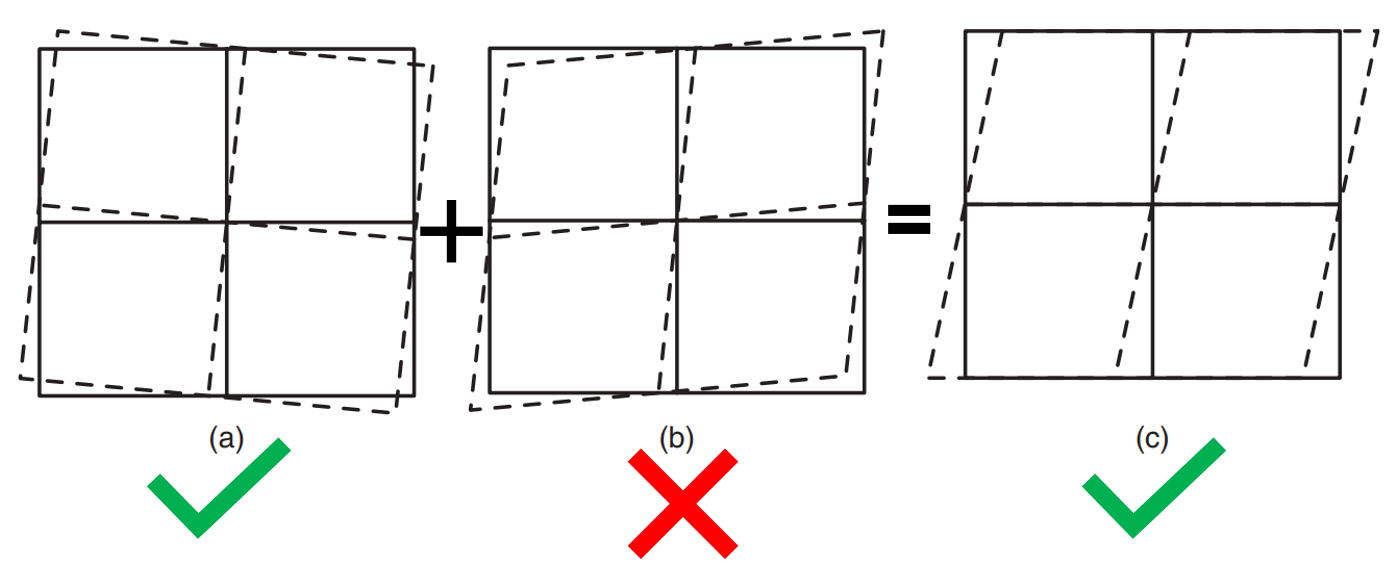
irrotationality
Irrotationality is a property of the flow (and not the fluid itself). The influence of this assumption is mathematically very apparent in that it leads to the fluid flow behavior to be represented using the Laplace’s equation. Which is an incredible simplification because of the properties that the function \(\phi\), that statisfies the Laplace equation, is bound to exhibit. This is a linear equation which means it is amenable to superposition - i.e. flowfield around two bodies placed close to each other is the sum of the flow fields of the two bodies in isolation. The function \(\phi\) is continuous and differentiable (referred to as holomorphic in mathematical parlance) which means any differentiable function represents the flow over some body! We just need to identify the function that represents the flowfield over the body of interest to us - an airfoil or a flat plate (airfoil with zero thickness). Lastly, and from the point of view of early practioners in the field of aerodynamics, the ubiquity with which this function appears in different areas of physics - electrostatics, gravitation etc. - means that aerodynamiscists would not be alone in their struggle to identify solution strategies for the Laplace’s equation.
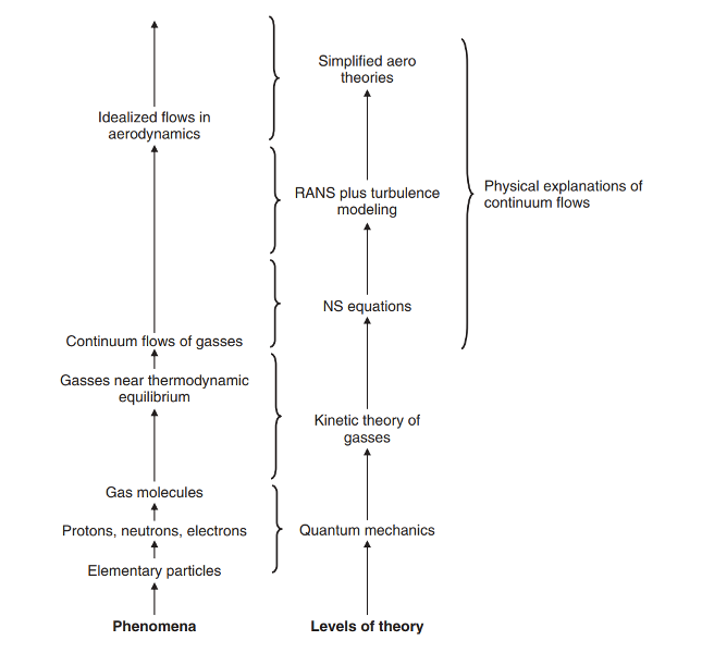
Heirarchy of physical theories [taken from "Understanding Aerodynamics" by Doug McLean] [source]
Principle aim of a model
include just relevant behavior of physical systems
superfluousness (generally) increases computational complexity
(too much) parsimony can make it useless
NSE are an approximate model of fluids
rarely do these approximations become limitations
fluids modelled as a continuous medium
granularity (individual molecules) is ignored
basic conservation laws are satisfied
mass, momentum, energy
constitutive relations between involved variables
to make as many equations as there are variables
Simple governing laws, complex results
The NSE are generally all that an aerospace engineer needs for all their aerodynamics analyses needs - five field partial differential equations and three constitutive relations to solve for three space coordinates (Lagrangian)/velocity components (Eulerian), pressure, density, temperature, viscosity and thermal conductivity. fuselage 1 Being field equations, the NSE can be solved if the boundary conditions of the domain of investigation are known. In case of boundaries that form the interface with another material - for e.g. the surface of a wing - additional conditions need to be imposed since NSE do not cover the physics at such interfaces. Examples include “no slip” boundary condition typically employed for flow over solid boundaries and “no temperature jump” in case of a temperature differential.
Since the momentum conservation equations are part of the NSE, Newton’s 2nd is definitely involved when describing flow behavior. However, simply attributing lift generated by an airfoil, for e.g., to just Newton’s 2nd law is not entirely accurate. There is an obvious cause and effect relation when one talks about Newton’s 2nd law. Within a fluid, however, the motion of continuum parcels is influenced by the forces exerted and the forces exerted are in turn influenced by the motion of these parcels. For e.g., the momentum equation above can be viewed as a form of Newton’s second law of motion F=mass x acceleration, except that the forcing terms on the RHS of the equation - the pressure gradient and the shear stresses - are themselves a function of the fluid velocity. The complex interaction between the three sets of forces - inertial, pressure and shear - is what gives fluid dynamics its richness.
Such implicit relations of relatively simple local physics (conservation laws) buried within the NSE make an intuitive foresight of what would happen in the global flowfield difficult. Below is an informal discussion of the mechanism by which airfoils generate lift to exemplify this.
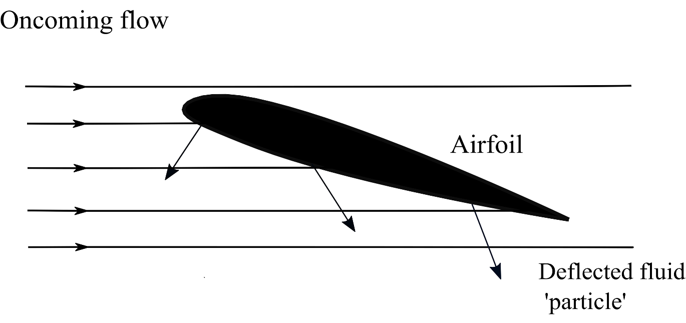
Streamlines representing hypothetical fluid flow idealised as independent fluid 'particles' (Newton's approach)
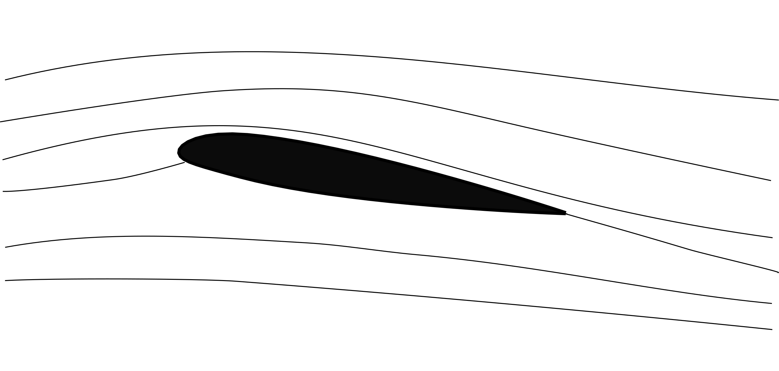
Streamlines representing real fluid flow
Some of the salient features of fluid behavior have been summarised below -
fluid (infinitely deformable) follows airfoil contour
a result of rapid random motion of molecules
this influences fluid velocity in a large region in the vicinity of airfoil
natural by-product of fluids behaving as continuous media
flow sped up on upper surface and slowed down on lower surface
so Bernoulli-based explanation of lift is correct (but not sufficient!)
most lift occurs due to suction pressure on upper side
airfoil shape has a significant effect on lift generated
this is completely ignored by Newton’s approach
mutual/reciprocal relation between pressure and velocity
pressure difference causes fluid acceleration
existence of pressure difference due velocity difference
inertia plays central role
air is light but at fast enough speeds, large enough mass can be influenced
magnitude of lift generated can be controlled
linear dependence in \(\alpha\)
square dependence in fluid velocity
amount of fluid influenced
downward momentum imparted
the above effects die down with distance from the airfoil surfaces
Aside
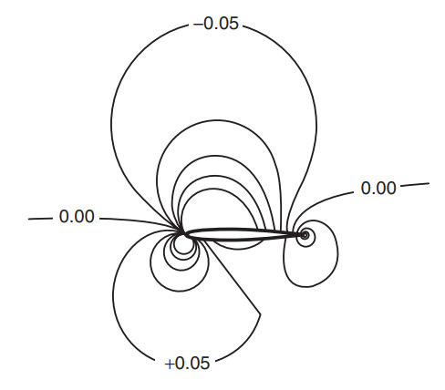
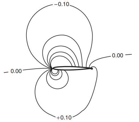
If the picture on the left above is assumed to be the true fluid model, then it is easy to see that the lift generated would be proportional to square of the angle of attack. However, we now know that airfoil lift is proportional to angle of attack (at least when the flow is not significantly separated). This is also evident from the pressure contours around an airfoil shown below - doubling the anlge of attack doubles the pressure difference, the amount of fluid influenced stays the same.
Notice that viscosity did not come up in explanation above. Viscosity plays a key role in the ability of airfoil sections to produce lift in that it ensures that the fluid doesn’t turn around the trailing edge. However, it is not necessary in order to quantify the amount of lift which is why simple potential flow theory models, such as thin airfoil theory, are capable to predicting airfoil lift to a good degree of accuracy. Even when the flow conditions are unsteady, potential flow theory-based unsteady models are just as capable in predicting the unsteady lift and moment variation.
Generation of lift
“Lift is an interaction in which the airfoil and the fluid exchange equal and opposite forces (as per Newton’s third law)” - [McL13].
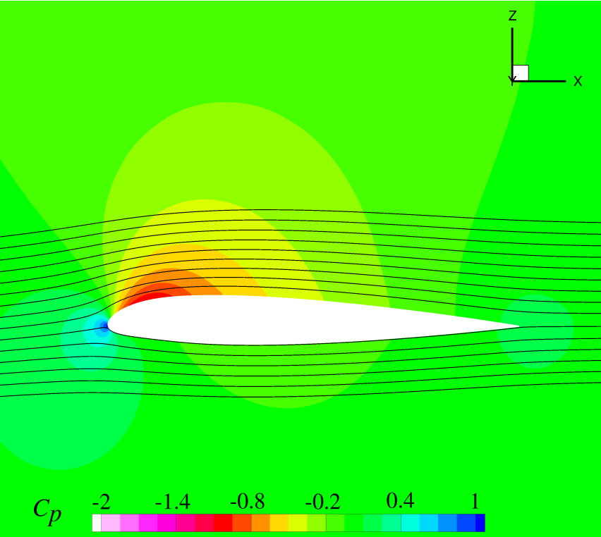
Coefficient of pressure contour plot of NACA23012 airfoil at $M=0.4$ and $\alpha = 2^°$ [source]
mathematically
its because of the NSE
intuitively
?
always accompanied by circulation and vorticity
manifests as pressure difference
envisaged as flow turning
below the airfoil AND above it!!
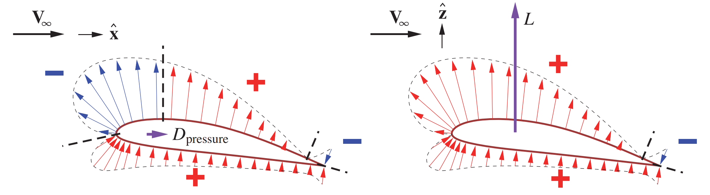
Pressure distribution around an airfoil that contributes to drag (left) and lift (right). Red arrows show positive contribution and blue arrows negative contribution. [source]
Vorticity and circulation
Vorticity \(\mathbf{\omega}\) is a measure of the local rotation of fluid elements i.e. the element rotation about its own axis. If the velocity flow field \(\mathbf{V}\) is known at every point then mathematically this ‘rotation’ can be quantified using the following equation -
Vorticity of a continuum particle/element (modified from [source])
Fluid dynamics, as it concerns aerospace engineering, is largely about keeping track of vorticity generation and vorticity transport. It is introduced into the flow due to no-slip condition at the airfoil surface (or the surface of any body for that matter). This vorticity doesn‘t just immediately dissipate/dissapear and keeping track of it is imperative to get overall aerodynamics right. Note that viscosity is not necessary in order to generate vorticity, based on the flow profiles shown above if somehow a velocity shear exists between two layers of fluid then we know from the definition that a sheet of vorticity exists between those two layers and viscosity does not even come into the picture.
Recall that the velocity profile within the boundary layer on the upper surface looks like that shown in figure (c) above, where the lower fluid layers always have a lower velocity than the ones above them leading to a shearing effect and consequently generate vorticity in the fluid. The figure below shows varying degrees of modelling fidelity where the vorticity distributed within the fluid volume in the boundary layer is approximated as lumped as a sheet over the surface of the airfoil itself or lumped over a line (usually the camber line of the airfoil). Alternately, the entire distributed circulatory effect of the airfoil can also be lumped at just one point on the airfoil (usually the quarter-chord). With each simplification the accuracy of the velocity field prediction is affected, especially close (within a few chord lengths) to the airfoil. However, for most applications (including rotary-wing analysis) representing the circulation around the airfoil as lumped at the quarter chord location suffices and modelling the wake of the blade (finite-wing) using Prandtl’s lifting-line theory becomes more relevant for accurate analysis.
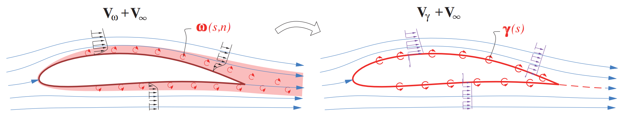
Schematic of the actual vorticity distribution around an airfoil due to the boundary layer and in the wake compared in real flow versus a simplified model [source]
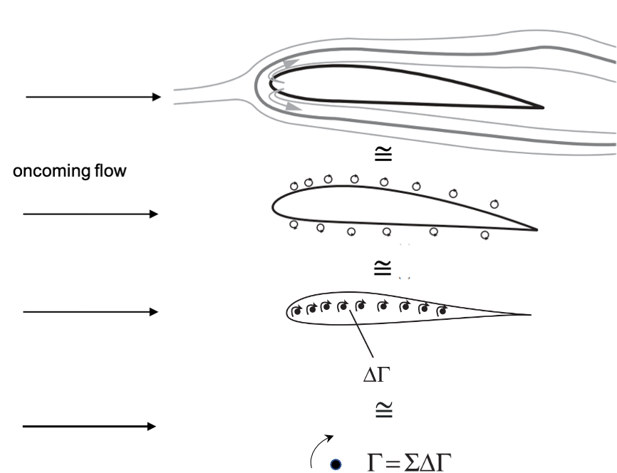
Schematic showing the origins of flow vorticity in the boundary layer and further levels of modelling fidelity (modified from [source])
The circulation of the flow is a relevant quantity because it quanitifies the amount of lift being generated per the Kutta-Joukowski theorem.
The following video presents some interesting experimental demonstrations that you might find useful to further help clarify the two concepts.
from IPython.display import YouTubeVideo
YouTubeVideo('pOA3VJHCnWs', width=800, height=400)
Potential flow theory
We are fixated quite a bit on the rotationality of the flow \(\nabla \times \mathbf{V}\), or its lack thereof. This is for a good reason. The irrotationality condition \(\nabla \times \mathbf{V} = 0\) guarantees the existence of a \(\phi\) such that \(\mathbf{V} = \nabla \phi\).
This, together with the continuity equation for an incompressible flow gives the Laplace’s equation \( \nabla^2 \phi = 0\). This is valid irrespective of whether the flow is unsteady and is true for both 2D and 3D representations. Alternately, if we begin with the incompressibility assumption \(\nabla.\mathbf{V} = 0\), then for the special case of 2D flow scenarios the irrotationality assumption allows the possibility of some function \(\psi\) such that it automatically satisfies the irrotationality condition.
Physically, \(\psi\) denotes a streamline in a flow and is called the stream function.
Not just that, the difference in the magnitude of \(\psi\) between two streamlines is related to the rate of mass flow of fluid between the two streamlines (for \(\rho\)=const).
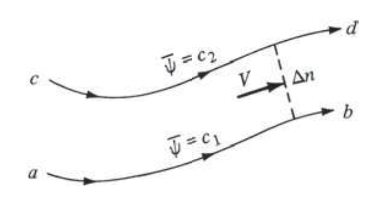
Flow between two streamlines. [source]
Note that \(\psi\) and \(\phi\) are not equivalent here. \(\psi\) can only be used for 2D flow representations and its form is coordinate dependent while \(\phi\) can be used for modelling 3D flows and is coordinate-free. Of course all of this is contingent on the continuity equation, which is a fundamental law of nature, and the irrotationality assumption. Its the latter condition that one needs to be mindfull of, since not all fluid flows satisfy that condition and potential flow theory based solutions would not be accurate in such scenarios. Fortunately, the assumption applies for attached flow around an airfoil (the experiment of Bryant and Williams [BW26] discussed below) and airfoils are the fundamental building blocks of most aerospace applications potential flow theory has developed into a viable theory for analysing flows.
Since \(\psi\) and \(\phi\) are different representation of the the velocity field itself, from the above discussion it follows that -
The above equations present a pair of Cauchy-Reimann Equations such that a complex function given by F(z = x+iy) is complex differentiable (infinitely differentiable) if it is given as -
The derivative is given as
where \(\bar{w}\) is the conjugate of the velocity in the complex domain.
Elementary flows
So posing the problem of a real-world fluid flow in abstract terms of complex analysis provides us the insight that the functions \(\psi\) and \(\phi\), which are used to represent real fluid flow velocities, are indeed continuous and infinitely differentiable everywhere in the domain. Additionally, \(F(z)\) also satisfies the Laplace’s equation since both \(\psi\) and \(\phi\) satisfy it.
This is a useful because the Laplace’s equation is linear. If the function \(F(z)\) can simply be evaluated for simple elementary flows and these elementary flows can be used to create the flow field around any complicated geometry then \(F(z)\) can be obtained essentially for any complicated geometry. Knowing \(F(z)\), the flow velocity around any geometry can be evaluated and thereafter using the Bernoulli’s equation to get the pressure distribution is a straightforward excercise. The question arises, what sort elementary flows are useful?
Uniform flow $\(F(z) = U_\infty z \)$
Uniform flow at an angle of attack \(\alpha\) $\(F(z) = U_\infty e^{-i\alpha} z \)$
Source/Sink $\(F(z) = \frac{m}{2\pi}\text{ln} z\)$
Line vortex $\(F(z) = \frac{\Gamma}{2\pi i}\text{ln} z\)$
Doublet $\(F(z) = \frac{\mu}{2\pi z}\)$
The elementary flow fields represented by the complex function \(F(z)\) satisfy the continuity equation as well as the irrotationality condition everywhere in the domain except at the point where the singularity exists. That is okay because the flow filed right at the point of singularity, or close to it, is not of interest to us.
Practical application from elementary solutions
Source+ image Source pair $\(F(z) = \frac{m}{2\pi}\text{ln} \frac{z+a}{z-a}\)$
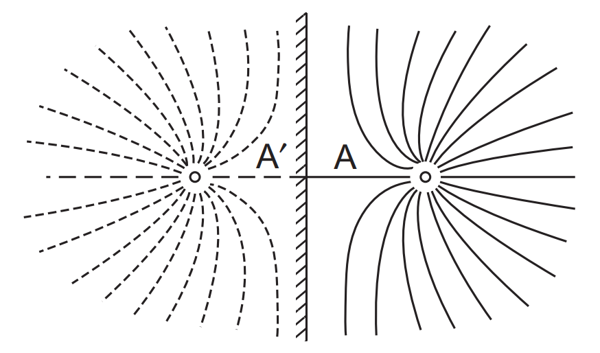
Solid wall modelled using the method of images. [source]
Source+Sink pair in horizontal flow $\(F(z) = \frac{-m}{2\pi}\text{ln} (z-a) + \frac{m}{2\pi}\text{ln} (z+a) + + U_\infty z\)$
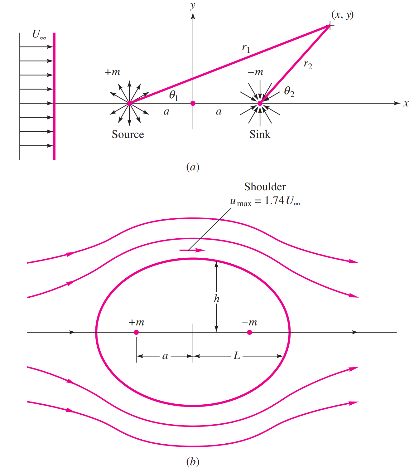
Flow around a Rankine body. [source]
Doublet in horizontal flow $\(F(z) = \frac{\mu}{2\pi z} + U_\infty z\)$
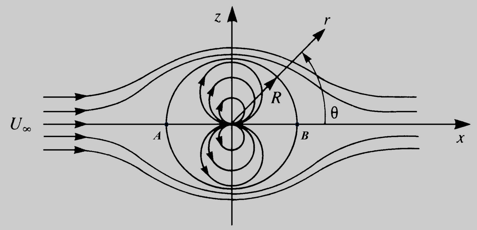
Flow around a circular cylinder. [source]
It is already shown above that \(F'(z)\) gives the complex conjugate of the complex velocity. So, once \(F(z)\) for any arbitrary geometry is constructed the complex derivative would give the velocity distribution around the body.
where \(V_r\) and \(V_\theta\) represent the radial and the tangential components of the flow velocity around the cylinder. In order to confirm that a doublet in a free stream indeed represents flow around a cyclinder, simply the no-penetration boundary condition should be satisfied, i.e. \(V_r(R)=0\).
The radius of the cylinder depends on the strength of the doublet as well as the free stream velocity combination used to construct the flow field. Usually, you’d want to model flow around a specific cylinder in a flow so \(R\) and \(U_\infty\) are known and \(\mu\) can be obtained by satisfying the no-penetration condition above. This gives-
Applying the Bernoulli’s equation, the pressure distribution around the cylinder can be obtained -
This pressure distribution results in a zero net lift and zero drag. The zero net lift and zero drag come from perfect fore-aft and top-down symmetry of the flow and the fact that viscosity is ignored in potential flow theory. Additionally, the stream function is given by the imaginary part of \(F(z)\).
The streamline \(\psi=0\) defines the boundary of the cylinder.
One of the early experiments by Fuhrmann and Prandtl involving flow around a slender airship-like body in a wind tunnel showed that indeed the measured pressure distribution around the body matched that predicted by theory [Blo19]. The theoretical pressure was obtained using potential flow theory where the geometry was modelled by placing multiple sinks and sources in a uniform flow as shown below.
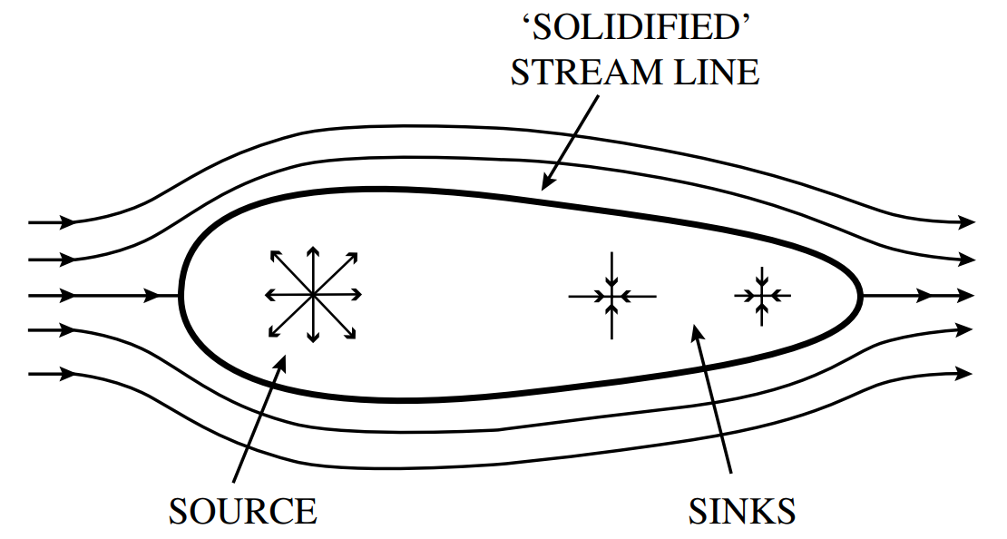
Fuhrmann and Prandtl study of a uniform flow around an airship-like solid body. [source])
Due to the low magnitude of kinematic viscosity (\(\nu/\rho\)) of air, most flows of interest to an aerospace engineer occur at high Reynolds numbers (>\(10^6\)) and low angles of attack \(\alpha\). In such conditions the flow can be modelled reasonably well by dropping the viscous terms (i.e. assuming \(\nu=0\), limiting case of a viscous fluid). Of course, one runs the risk of not being able to model effects of flow separation (which are viscous in nature), viscous drag etc. But the speed and ease of solving the fluid flow equations assuming \(\nu=0\) as well as the physicality of the results has led to the popularity of the potential flow theory. Even extensions to this theory have been proposed that account for the viscous effects in some adhoc way but without having to solve the full NSE equations. In fact for low Mach number flows, the fluid equations can be further simplified and yet be physically representative of the real flow field.
When the irrotationality and the incompressibilty assumptions are made along with zero viscosity, the NSE reduce to two eqs - the Laplacian and the Bernoulli’s eq.
Here \(\phi\) is some unknown function that needs to be found out and all the quantities of interest in the entire flowfield would be known. \(\rho\) is a constant quantity that is known apriori, if the Laplacian can be solved i.e. \(\phi\) is obtained over the entire fluid domain then the fluid velocity can be obtained using the following relation -
This is highly convenient because \(\phi\) is a scalar function, only one known quantity at a given coordinate location, but velocity has three components at each point that need to be found out. Additionally, \(\phi\) is independent of the coordinate system and, based on the form of the \(\nabla\) operator, the velocity vector \(\mathbf{V}\) can be evaluated in any coordinate system.2
the early go-to model for obtaining pressure distribution of slender bodies
airfoils, airships etc.
bodies of any shape could be analysed
conformal theory used to obtain analytic results of pressure distribution
also used in unsteady aerodynamic theories - for e.g. Theodorsen theory
The potential flow theory discussion above is partially based on the details presented in [Sen14](Chapter 3). Students interested in the derivation of some of the results presented above can refer this source.
Kutta-Joukowski theorem
Addition of a line vortex doesn’t disturb the cylindrical geometry established by the doublet+uniform flow combination. However, the flow around the cylinder is changed dramatically so much so that now when the integrated effect of the pressure distribution is evaluated a non-zero lift exists. The drag force is still zero. Intuitively this makes sense because the flow is no longer has a top-down symmetry. Instead, a clockwise circulation leads to higher flow velocity at the upper surface of the cylinder and flow slows down at the lower surface. We know from the Bernoulli’s relation that this should lead to lower pressure at the top and higher pressure at the bottom.
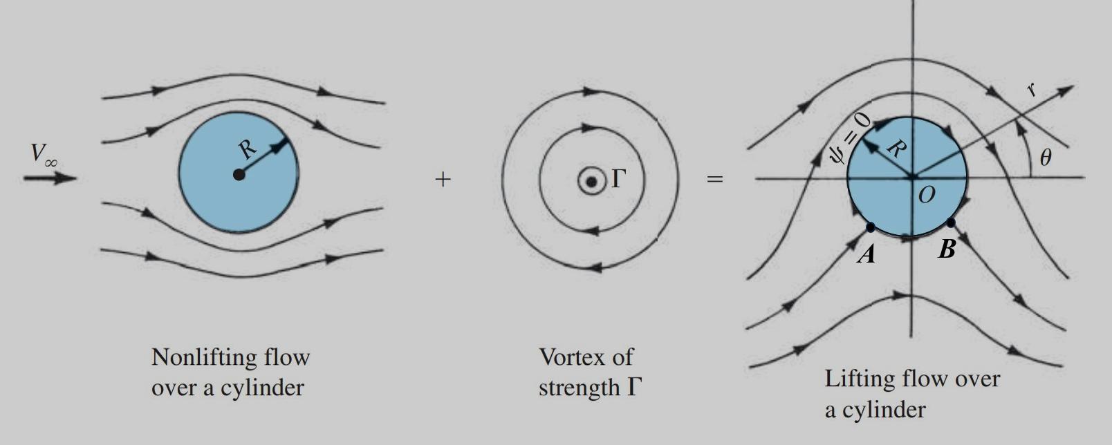
Flow around a circular cylinder with circulation. [source]
Clearly, if indeed there is lift generated in the above case it has to be related to the circulation strength \(\Gamma\). In fact, if carry out the same excercise as the non-lifting cylinder case discussed earlier, the amount of lift generated (per unit length since its 2D) turns out to be -
This result leads to the more general case that the lifting force generated by any entity in an incompressible, inviscid, irrotational flow in an unbounded fluid is proportional to the circulation around it and perpendicular to the oncoming flow velocity direction. This relation is a consequence of the Kutta-Joukowski theorem. A more general notation for identifying the direction of resultant force using the Kutta-Joukowski theorem can be obtained by defining the direction of \(\Gamma\) as a vector quantity based on the right hand rule and using the following relation to give the resultant lift force per unit span (\(\mathbf{Q}_{\infty}=\mathbf{V}_{\infty}\)) -
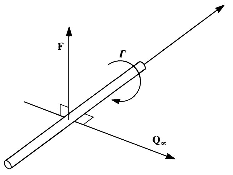
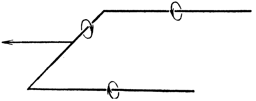
Vector notation for Kutta-Joukowski theorem ([source])
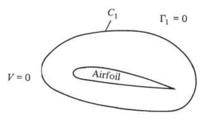
This relation tells us the simple fact that lift is related to the circulation around the body in question. So if the circulation were zero, there would be no lift generated. On the other hand, if you knew precisely the circulation around the cross-section of cylinder, or more practical entities of interest such as a wing or a blade, you could get the lift per unit span and the total lift would simply be an integral over all such sections over its span. Precise experiments carried out in the wind tunnel by Bryant and Williams [BW26] with wing sections, where the flow velocities around these section have been measured, show that indeed the effect of an airfoil is to introduce a circulation around itself and that circulation everywhere else in the fluid domain is zero, or rather close to zero, such that the potential flow theory assumption of irrotational flow is not misplaced.
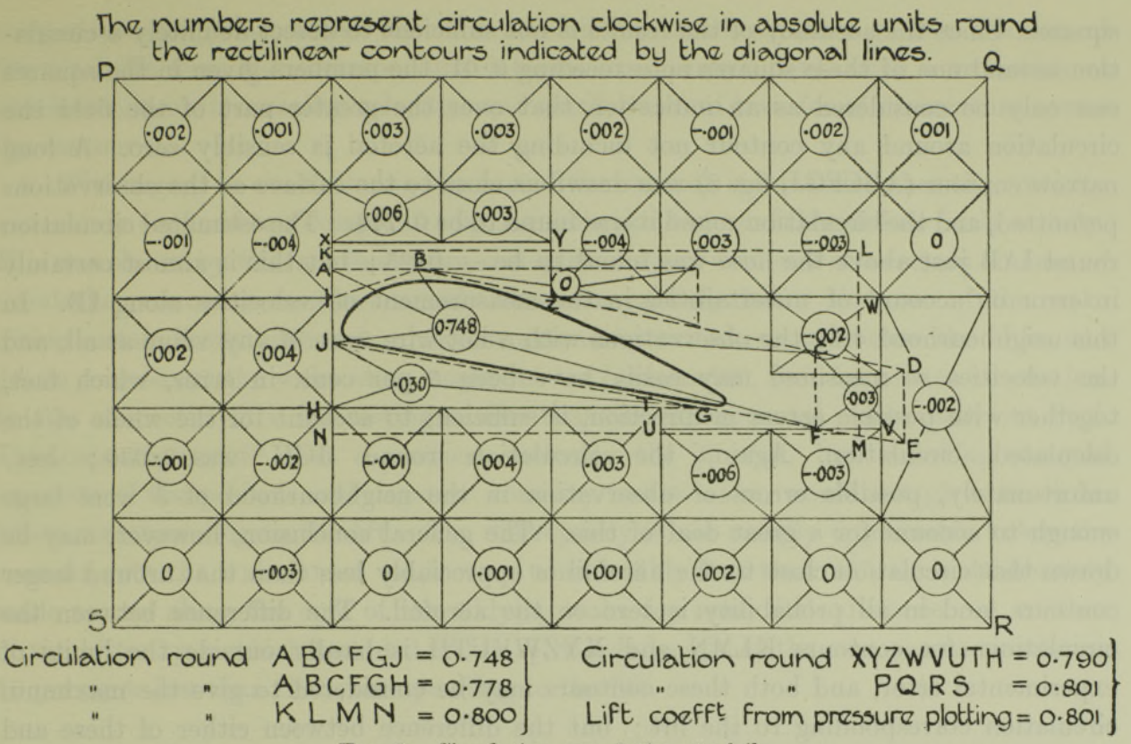
Schematic of the experimentally measured circulation around an airfoil section [source]
Note that the contours used in the experiments of Bryant and Williams were perpendicular to the wake of the airfoil. This is to ensure that that the effect of the vorticity in the wake of the airfoil is not included in the circulation measurement around the airfoil.
Kutta condition
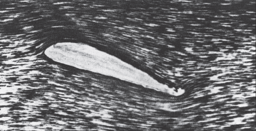
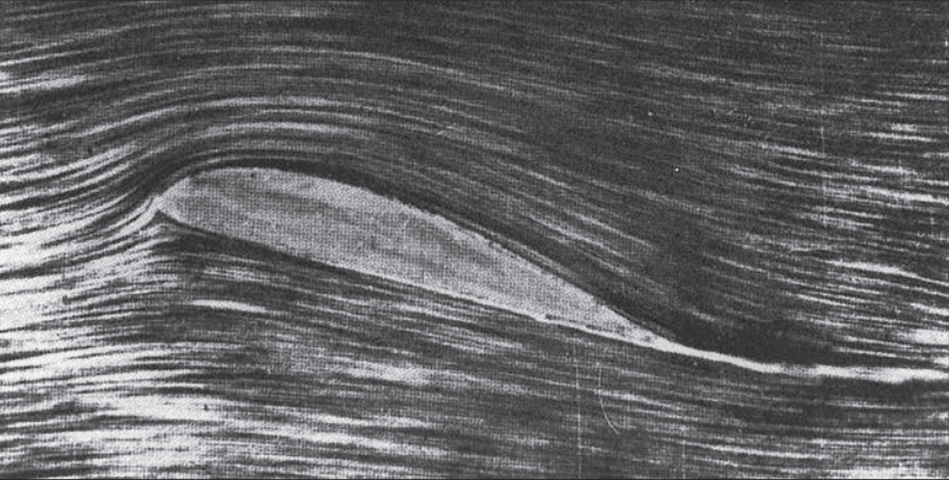
Based on the potential flow theory, lift generation can be predicted using a simple relation given by the Kutta-Joukowski theorem. This raises the natural question, how does one obtain \(\Gamma\)!? Potential flow theory, on its own cannot uniquely predict the amount of lift an airfoil is capable of generating. Since the amount of circulation in the flow is undecided, some more physics needs to be modelled in order to account for this. We could either go to the origins of the potential flow theory and see if some of the assumptions made can be relaxed to include more physics for this purpose. This is bound to make the equations more involved that the Laplace equation. Alternately, this is done using the Kutta condition. To illustrate the situation schematically, consider the two flow representations shown below for the same \(\alpha\) and \(V_{\infty}\) but different circulations around the airfoils. Both are valid/possible within the framework of potential flow theory, which one is correct?
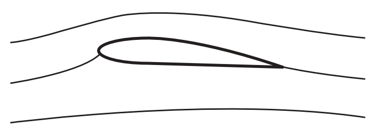
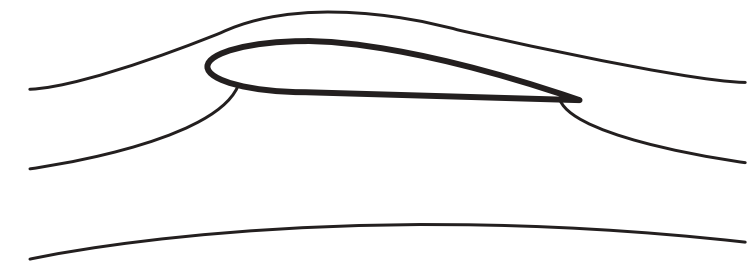
Streamlines around an airfoil (real flow) [source]
Streamlines representation around an airfoil based on a mathematically valid potential flow solution (not a real flow) [source])
In reality, only the one on the left is observed. This is a consequence of the viscosity of fluids in nature and the fact that they cannot turn around sharp corners (airfoil trailing edges are sharp enough). Since potential flow theory doesn’t model viscosity, a condition needs to be mathematically enforced so that the resulting flow field obtained is physically correct and unique3. This is achieved by enforcing what is called the Kutta condition. Based on what your favorite reference textbook for fluid dynamics is, this could also be referred to as the Joukowski condition [RL13].
Instantaneous flow field just from impulsive start of airfoil [source]
Steady state flow field around an airfoil [source])
Potential flow theory alone cannot determine the amount of circulation around a body. This is true in the case of steady as well as unsteady aerodynamics. Even the widely used thin airfoil theory results of the lift curve slope=\(2\pi\), \(C_{m_{c/4}}=0\) etc. are obtained after imposing an additional condition based on the flow physics. Purely following the mathematical construct of potential flow theory would not give us a unique solution (and hence no solution). The amount of circulation decides where the stagnation points would be. The Kutta condition tells us where the stagnation points ought to be in the case of flow around an airfoil. Therefore, by extension it helps identify a unique circulation that exists around an airfoil at a given angle of attack.
The Kutta condition is an engineering approximation that is based on experimental observations rather than mathematically derived from first principles. Images of flow field development taken at the instant flow is started around an airfoil suggest that there some flow turning occurs at the airfoil trailing edge but large shear forces encountered quickly make the flow pass smoothly at the trailing edge rather than turn around it. The Kutta condition is an indispensable part of introductory aerodynamics textbooks owing to the success of potential flow theory together with this empirically observed assumption.
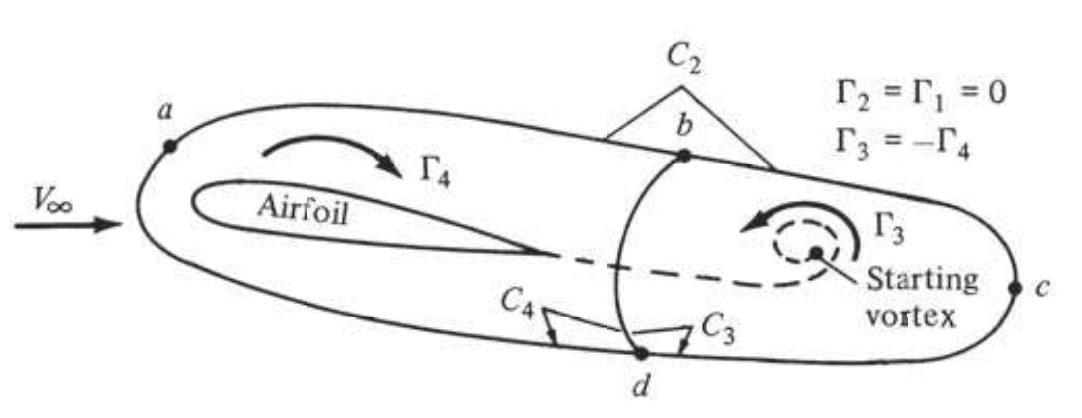
Kelvin’s circulation theorem
For an inviscid, incompressible fluid of constant density, the circulation around any closed loop within the fluid remains time-invariant. For an airfoil initially at rest within a fluid, the circulation around any contour within the fluid is going to be zero. When the fluid is set in motion there is vorticity due to the uniform fluid velocity, yet we now know (from the discussion aboce) that there would be a circulation set around the airfoil. The Kelvin’s circulation theorem implies that a vorticity of opposite sign must be getting introduced in the fluid so that the net circulation around any closed contour, that includes the airfoil in it, must be zero. The video below demonstrates this perfectly. A series of stillshots from the video above are also available in [TtranslatorH34].
from IPython.display import YouTubeVideo
YouTubeVideo('VcggiVSf5F8', width=800, height=400)
Zero circulation in a fluid at rest ([source])
Starting vortex observed behind an airfoil in a fluid ([source])
Section 9.4 in [Gla36] presents a concise and clear explanation of the development of the bound and starting vortices and the interested students are encouraged to read the relevant couple of pages for this reference.
3D aerodynamics
The validity of Prandtl’s theory of circulation was established for the 2D airfoil (infinite wing) case by experiments conducted by Bryant and Williams [BW26]. The corresponding verification tests for the finite-wing case were conducted by Fage and Simmons [FS26]. This is shown schematically below where flowfield velocity measurements were carried out in 4 different planes (A, B, C and D) before and after the wing.
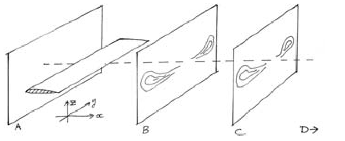
Schematic representation of flow profiles behind a finite wing [source]
Schematic of the experimentally measured circulation around an airfoil section [source]
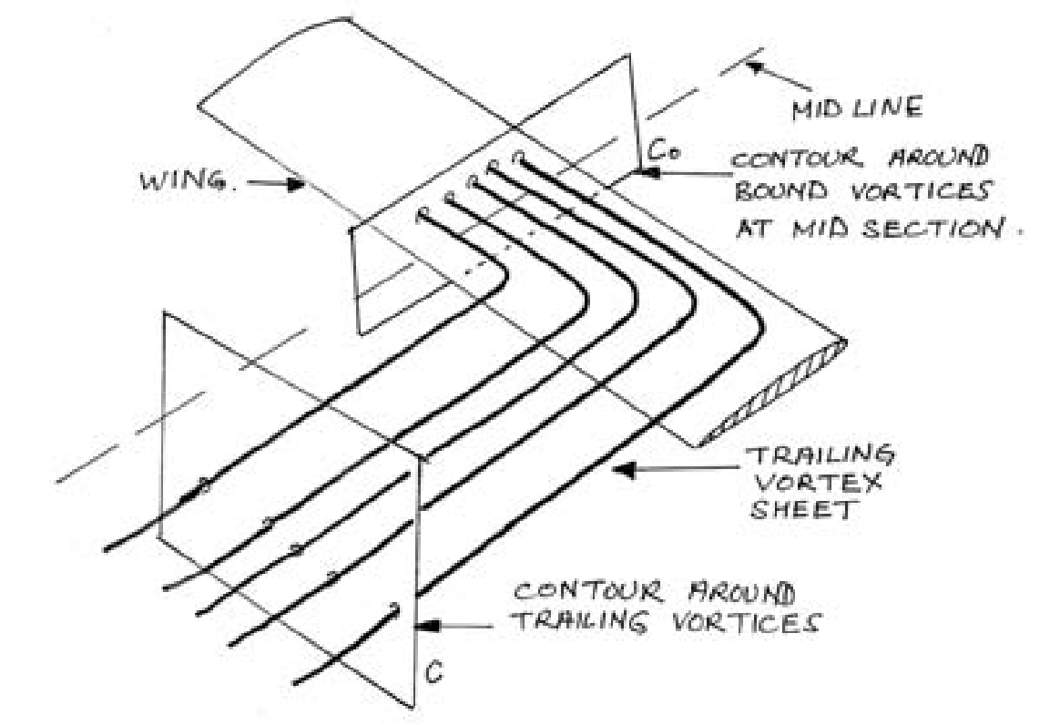
The contours \(C\) and \(C_o\) are seemingly unrelated as far as the flow field is concerned. However, if Prandtl’s lifting line theory is to be believed then the circulation about the two contours should be equal. Additionally, since the circulation about \(C_o\) represents bound circulation, it is related to the lifting force generated by the wing -
where \(\Gamma_b\) is the circulation due to vorticity bound to the wing, \(V\) is the oncoming flow velocity, \(S\) is the area of the wing and \(b\) is its span. Based on their meticulous flow field measurements using a hot wire probe, Fage and Simmons showed all the above assertions to be true. The two experiments of [BW26] and [BW26] had helped establish that indeed the theory of circulation conformed with reality.
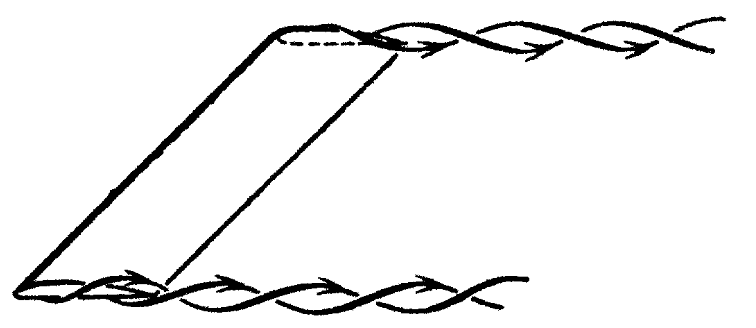
Tip vortices generated at the wing tips of a finite wing [source]
Modelling a finite wing using bound and trailing vortices [source]
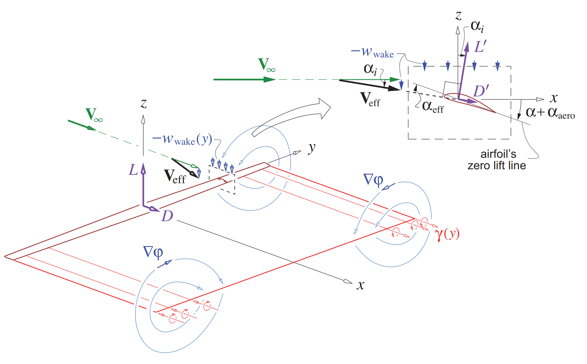
Source of induced velocity on a finite-wing using Prandtl's lifting-line theory [source]
As [Joh13] puts it - ‘Blade element theory is essentially lifting-line theory for the rotary wing.’ (Section 9.2).
Final Comments
The above, seemingly dissociated, set of concepts are nothing new and have been covered at length in fundamental fluid dynamics courses. These would all be used in order to build the framework for unsteady aerodynamics analyses.
One thing worth emphasising again before moving on is that the Kutta condition is an engineering condition that is imposed on the flow in order to obtain deterministic properties of lift and moment around an airfoil. It is not derived mathematically from first principles. While it has successfully been used for steady airfoil analysis, unsteady airfoil analysis presents a challenge because experimental observations suggest that indeed the flow can briefly turn around the airfoil trailing-edge when rapid motion is involved. So the Kutta condition isn’t strictly applicable for unsteady flows [TR19]. Neither is it helpful for cases when a sharp edge doesn’t exist, for e.g. the airship-like body from the tests of Fuhrmann and Prandtl above, or when more than one sharp edges exist for some random profile (i.e. not necessarily an airfoil-like profile). However, early unsteady airfoil theory was developed accepting the validity of the Kutta condition even for unsteady airfoil motion and has been shown to provide acceptable prediction of unsteady airfoil lift and moments.
Potential flow theory-based results remain meaningful only in when the flow remains attached to the airfoil. In flow conditions where there is large scale separation, the linearity imposed on the solutions by the potential flow theory introduces inaccuracies. If you are still wondering, how on Earth does a flow model based on zero viscosity give results that are representative of viscous real-world flows well you are not alone since some of the brightest minds of the 20th century struggled with the same ideas. This struggle is chronicled in [Blo19] as a clash between the British and the German school of aerodynamicists. The theories proposed by the latter school were eventually universally accepted once supporting experimental evidence was obtained and the entire saga has been artfully concluded in the final passages of [Blo19].
David Bloor in ‘Enigma of the Aerofoil’
The German advances in the understanding of lift and the properties of wings depended on the use of abstract and unreal concepts that were sometimes employed with questionable logic. Progress in aerodynamics thus depended on the triumph of falsity over truth. Everyone knows that false premises can sometimes lead to true conclusions and that evidence can sometimes support false theories, but the story of the aerofoil involved more than this. The successful strategy involved the deliberate use of known falsehoods poised in artful balance with accepted truths. The supporters of the theory of circulation showed how simple falsehoods could yield dependable conclusions when dealing with a complex and otherwise intractable reality. This is the real enigma of the aerofoil… The enigma of the aerofoil is the enigma of all knowledge.
- 1
When modelling rotor wake there is not much to be gained from solving the most complex form of the problem. For e.g., most rotorcraft (atleast conventional designs) don’t fly faster than M=0.3 so right away density can be assumed to be constant without incurring much error. So can temperature and viscosity, and thermal conductivity is just zero. From the continuity and the momentum conservation equations, the problem then boils down to solving for the three velocity components and the pressure distribution. More on that later.
- 2
For most applications the gradient of the potential function \(\phi\) is evaluated in the cartesian coordinates. However, finite-state inflow models exist (also called dynamic inflow models) where the induced flow of a rotor is evaluated using a potential flow theory-based solution of the rotor. Here, the Laplacian is solved in ellipsoidal coordinates because the problem is amenable to an analytical solution in such a system. One of the most common such inflow model used extensively in real-time rotor simulations is the Peter-He inflow model.
- 3
Recall that we carried out a similar excercise when we ignored the negative root of the quadratic induced flow velocity equation.