Theodorsen Theory
Contents
Theodorsen Theory
“…why linear systems are so important. The answer is simple: because we can solve them!”
Theodore Theodorsen was first to publish a complete and detailed solution to the problem of aerodynamic loads on an oscillating lifting surface. Chapter 5 in [BAH96] is a great resource for understanding the theoretical foundations of the Theodorsen model (even better than the original paper by Dr Theodorsen that describes the model [The40]). That said, the complete derivation is mathematically involved and requires meticulously solving a lot of complex-valued integrals. Here we will start with the final results proposed by Theodorsen and work our way to backwards with the motivation to understand the expressions involved intuitively and take assummptions involved at face value.
The Theodorsen theory, or alternately the Theodorsen model, has been developed in the frequency domain i.e. the variable of interest is the frequency of input. The input in this case refers to the frequency at which the airfoil is moving. The Theodorsen theory only accounts for the pitching and heaving motions of the airfoil. The lead-lag motion of the airfoil, or alternately the variation in the oncoming flow velocity is not accounted for.
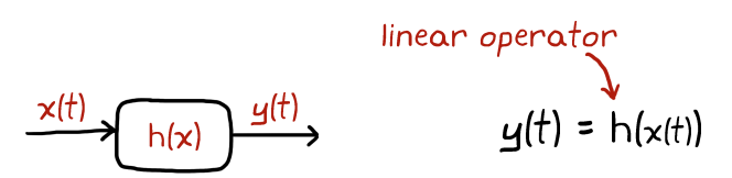
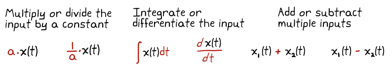
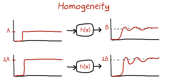
Aside: Linear time-invariant systems (LTI)
The behavior of a dynamical system ccan be mathematically represented using the input forcing \(x(t)\), the output response \(y(t)\) and the operator \(h\) that operates on the input.
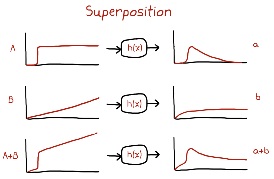
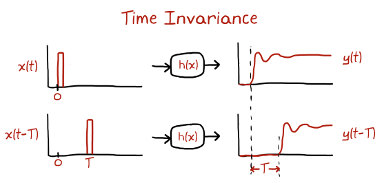
The discussion above and all the corresponding figures have been obtained from
.Aside: Frequency Response
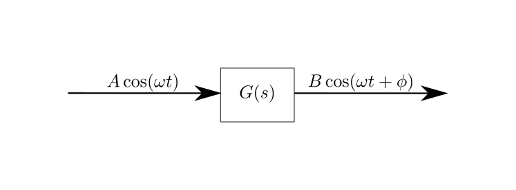
In the analysis of dynamical systems there has been sufficient progress so much so that there are multiple domains of modelling strategies that are available for one to choose from - frequency response, state-space, time-domain and impulse response. All these strategies apply to linear systems only and are equivalent in that any one form can be obtained from any one of the other forms. Dynamical systems are often studied in the frequency domain because the linearity assumption means that solving for the system response becomes especially straightforward once the transfer function \(G(s)\) of the system is known. \(G(s)\) relates the input forcing of the system at a given frequency to the output response of the system at the same frequency but now at a different amplitude as well as a phase shift.
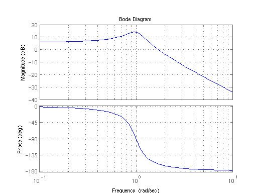
Bode plot [source]
Mathematical formulation
Airfoil+trailing-edge flap model in Theodorsen model [source]
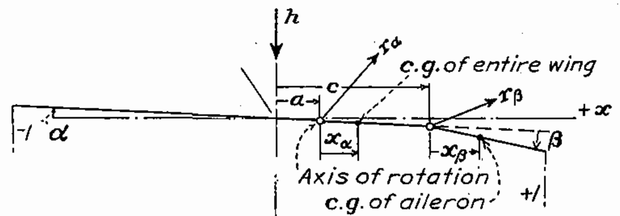
The schematic model of the airfoil with trailing-edge used in the Theodorsen model is shown above. The airfoil is placed such that the origin coincides with the mid-chord of the airfoil. The total chord length is \(2b\) where \(b\) is referred to as the semi-chord. This is done because quite often it is the semi-chord that keeps popping up in expressions rather than the total chord itself. The symbol \(c\) is reserved for the distance of the flap hinge from the mid-chord. The oncoming flow velocity is assumed to be constant within Theodorsen model and only steady-state aerodynamic pressure distribution over the airfoil due harmonic motion can be solved - no transients allowed. The centers of gravity of the airfoil and the trailing-edge flap are relevant here because Theodorsen went on to use the results of the model to analyse flutter.
Final equations
The total lift acting on the complete airfoil (i.e. together with flap) is
Moment acting about the airfoil pitching location \(x=ba\) is
The final equations are a result of the airfoil kinematics and the complex valued function \(C(k)\), commonly referred to as the Theodorsen function in literature. The former invloves reactionary loads experienced by the moving airfoil from pushing the fluid around and the latter manifests the time history of the oscillation, thereby incorporating hysteresis (effects of the history of motion) in the aerodynamic loads experienced by an airfoil. While the Theordorsen model involves an airfoil with trailing-edge flap, for simplicity we would look at the derivation below only for the case of an airfoil, i.e. no \(\beta\) terms. Note that the \(T_n\) terms are all attached to the \(\beta\) terms so we need not be focussed on what those are but for the curious minded these are different integrals that are laid down in Ref [The40].
Relevant building blocks
Understanding the Theodorsen theory requires a refresher of a number of theoretical aerodynamics concepts.
Potential flow theory
Kutta condition
No-penetration boundary condition
Conservation of circulation
Conformal mapping
Joukowski transformation
Unsteady Bernoulli’s equation
All these concepts have already been discussed in sufficient detail so that we can start using them now for the practical problem of an oscillating airfoil.
Non-circulatory lift
So the problem boils down to solving the Laplacian for the flow around a circular cross-section and then using the conformal mapping to obtain the flow around the thin airfoil profile. Thereafter, once the potential function in the z-plane is obtained only the corresponding potential function value at the airfoil surface is of interest since it, and its derivates, are directly related to the aerodynamic pressure forces using the unsteady Bernoulli’s equation. The pressure forces can be integrated over the entire airfoil to obtain lift force and moment about the quarter chord.
Potential flow theory and conformal mapping
The Theodorsen’s model begins with the conformal representation of a flat plate (airfoil) as a circle. The idea is to place sources/sinks around the circle so that a streamline is obtained that imitates flow around a circle (2D cylinder) placed in a fluid. Thereafter, using conformal mapping techniques, the fluid velocity distribution around the airfoil can be obtained.
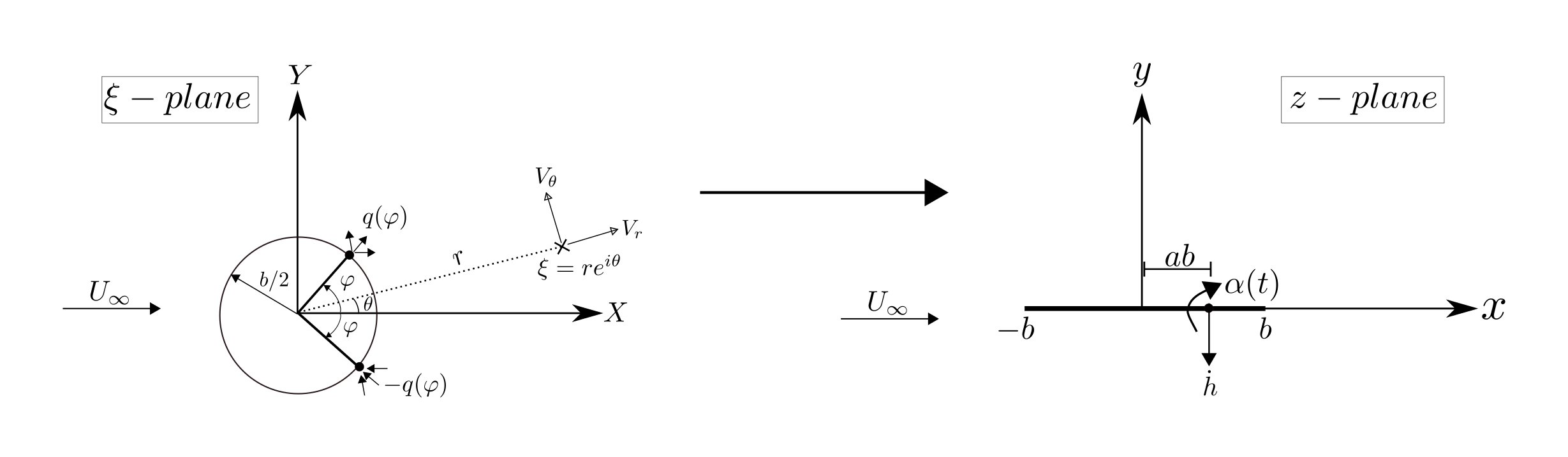
Theodorsen begins by placing sources in the upper half of the cylinder and sinks of equal strength in the lower half placed symmetrically about X-axis as shown below. This maps onto the \(z\)-plane at a single location (\(x\),0). Given the nature of the Joukowski transformation, and without going into further details, the source/sink pair doesn’t simply cancel the effect of each other.
Conformal representation of sources/sinks in the $\xi$-plane and the $z$-plane.
Recall that the complex function \(F(\xi)\) can be written down for the case of a source/sink. In case the source/sink is not exactly as the origin, an offset can be applied as
The corresponding velocity in the complex plane at some location \(re^{i\theta}\) off the cylinder is
where \(\xi=re^{i\theta}\), \(dV_{r}\) and \(dV_{\theta}\) denote the contribution to \(V_r\) and \(V_\theta\) at location \(\xi\) due to the source/sink pair on the circle at \(\frac{b}{2}e^{i\varphi}\) and \(\frac{b}{2}e^{-i\varphi}\). An integration over all such source/sink pairs over the entire cylinder will give the net radial and tangential flow velocities at any point in the domain. In particular, the tangential flow velocity at the cylinder surface i.e. at \(r=\frac{b}{2}\) simplifies to
Similarly, the expression for \(V_r(\frac{b}{2},\theta)\) can be obtained but some additional treatment is required so only the final expression will be stated here. Those interested in the details can check out Ref [BAH96] (Section 5-6).
So, based on som unknown distribution of sources and sinks \(q(\theta)\) on the cylinder surface, velocity distribution in the entire domain can be obtained including the surface of the cylinder itself. Much like the case of a doublet in a flow, we can obtain \(q(\theta)\) by satisfying the condition that normal flow at the boundary of the cylinder is zero.
No-penetration boundary condition
The velocity field at the cylinder surface is a function of the source/sink distribution strength \(q(\theta)\). This is an unknown quantity but knowledge about the motion of the airfoil can help arrive at a unique distribution using the no-penetration boundary condition.
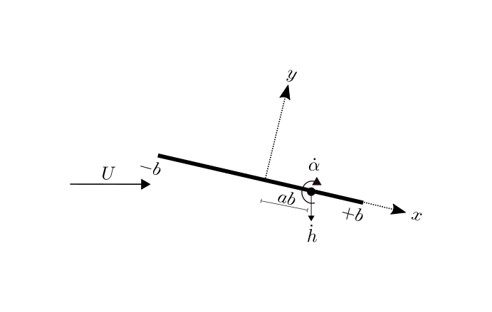
Representative airfoil motion involving pitching and plunging together with forward motion.
In the airfoil domain, the velocity normal to the airfoil surface due to its motion is given by
Theodorsen theory is concerned with only small motions of the airfoil such that the small angle approximation can be applied.
This is related to the radial velocity in the \(\xi\) domain on the surface of the cylinder by the relation-
Putting it all together
Once the distribution of source/sinks is known around the cylinder, based on the motion of the airfoil, then the tangential flow velocity at the cylinder surface \(V_\theta(\frac{b}{2},\theta)\) can be evaluated
Substituting for \(v_motion\) brings the integral in the form of the so called Galuert’s integral \(I_n\), commonly used in thin airfoil theory results, provided in [Gla36](Pg 92-93).
Again skipping the intermediate steps, the final result obtained as a consequence of carrying out the above integration is as follows-
Recall from the last chapter that,
We now have all the elements for obtaining lift generated by the airfoil undergoing \(V_{motion}\). But before solving for the expression of total lift we need \(\phi\) at the trailing-edge and \(\frac{\partial \phi}{\partial t}\)
Note that the Theodorsen theory assumes a constant oncoming flow velocity \(U\), however if the oncoming flow velocity is also time-varying then the above expression for \(\frac{\partial \phi}{\partial t}\) changes accordingly. Recall that a general airfoil section on rotor blade undergoes pitching, plunging and lead-lag motion so a general unsteady model that incorporates time-varying oncoming flow velocity is more relevant for rotocraft applications. Additionally, during forward flight motion there is a large time-varying component of the oncoming flow velocity too. Such a model exists and was proposed by Greenberg [Gre47] a few years after the Theodorsen’s model. However we continue to focus on the Theodorsen model for its relative simplicity.
From the last chapter, recall that
From the expression for \(\phi(\theta)\), we can see that for points on the surface of the cylinder that form a mirror image about the \(X\) axis, the potential functions at the two points are related by
Therefore the total lift generated over the airfoil surface spanning from \(-b\) to \(+b\) is given by-
Again, assuming \(\phi_{LE}=0\) the lift expression simplifies to
what we’ve ended up with is the non-circulatory component of lift i.e. aerodynamic force perpendicular to the oncoming flow that is not due to circulation. Here we start differentiating this from the total lift \(L\) by denoting this using \(L_{NC}\)
Salient features of \(L_{NC}\)
Circulation not needed for lift when unsteadiness involved
only sources/sinks distribution lead to \(L_{NC}\)
\(L_{NC}=0\) if \(\frac{\partial \phi}{\partial t}=0\)
Also refered to as lift due to added mass
\(L_{NC} = \underbrace{\pi \rho b^2}_\text{added mass} \underbrace{\left[(U \dot{\alpha}+\ddot{h}-\ddot{\alpha} a b) \right]}_\text{acceleration at mid-chord}\)due to acceleration of surrounding fluid as the airfoil moves
the amount of fluid influenced depends on size of airfoil
\(L_{NC}\) is the reactionary inertial force acted on the airfoil by the fluid
airfoil lift acts opposite to the direction of airfoil acceleration
Net \(L_{NC}\) over one actuation cycle is 0
There are some additional results worth noting based on the derivation so far. The velocity in the cylinder domain at the point corresponding to the airfoil trailing-edge is given by
Alternately,
This is a problem because we’ve ended up with an unphysical result at the trailing-edge. But this is no cause for concern yet because the lift generated from the circulatory component of flow has not been accounted for yet and this ‘issue’ can perhaps be fixed afterall.
Circulatory lift
Next we quantify the lift generated as a consequence of circulation around the airfoil.
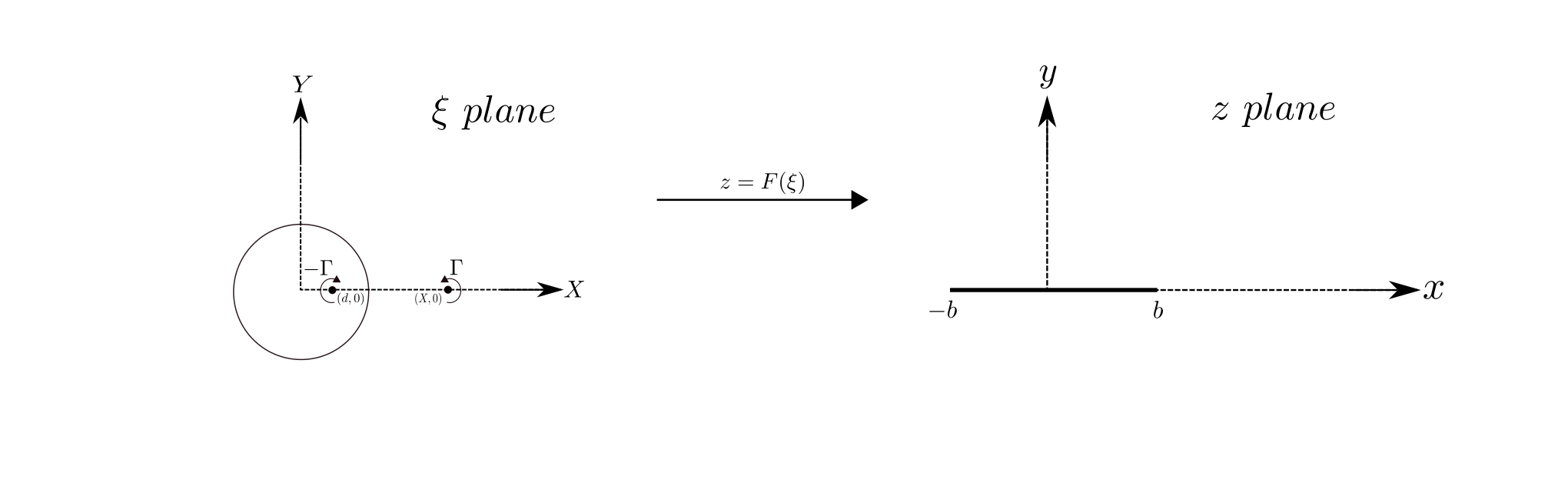
Conformal representation of vortices in the $\xi$-plane and the $z$-plane.
Conservation of circulation
That the dominant mechanism of lift generation by an airfoil is by introducing circulation has already been discussed. Any change in this circulation proceeds with shedding of an equivalent vortex of opposite strength in the wake that then moves away from the airfoil with the freestream. So clearly one needs to solve the flowfield for the situation when there is a vortex in the wake. We do this in the cylinder domain but now care needs to be taken because the addition of vortices that do not lie at the center of the cylinder as a streamline already established via placement of sources/sinks.
No-penetration boundary condition
The no-penetration boundary condition was already satisfied when solving for the non-circulatory flow. In the Theodorsen’s model this boundary condition is continued to be satisfied by judicious placement of \(-\Gamma\) such that the surface of the cylinder continues to be a streamline i.e. there is no flow perpendicular to it. The distance from the center of cylinder where the vortex needs to be placed is
Again, the detailed derivation is skipped in the interest of conciseness.
Kutta condition
The vortex strength \(\Gamma\) is unknown but in order for the Kutta condition to be satisfied at the trailing edge, i.e. \(u_{TE}\) is finite, the only possibility is that \(V_\theta(\frac{b}{2},0) = 0\) i.e.
Putting it all together
From the complex velocity conjugate result above, the required \(d\) that maintains the cylinder as a streamline is obtained using \(V_r=0\). However, we’ve already stated this result to be \(d = \frac{b^2}{4X}\). This gives the tangential flow velocity due to the pair of vortices
Using the Joukowski transformation expression the corresponding expression for tangential flow velocity using the coordinates of the vortex in the airfoil domain becomes
further considering the fact that in case of unsteady motion of the airfoil instead of a discrete starting vortex-like wake there would exist a distribution of vorticity \(\gamma(z,t)\),
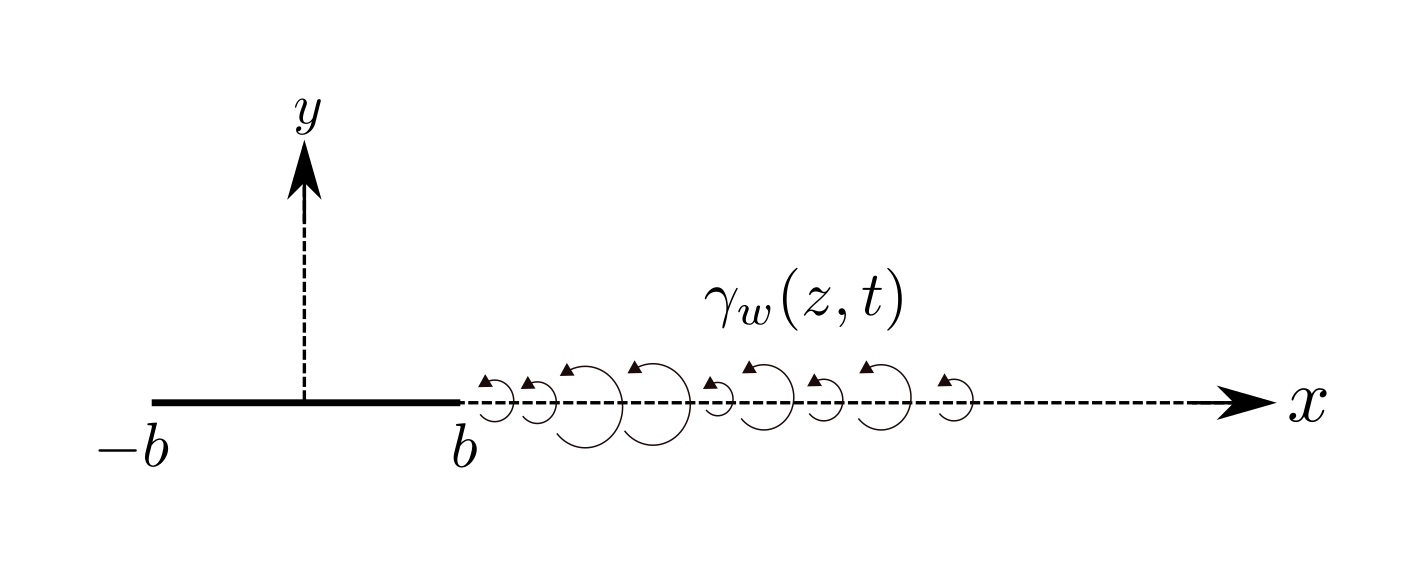
Conformal representation of a flat plate (airfoil) as a circle within the Theodorsen model.
Much like the steady aerodynamics case, the Kutta condition in the unsteady aerodynamics case needs to be satisfied which takes the form
This can be alternately written as
This is the integral circulation equation. The quantity on the RHS is known (since the motion of the airfoil is known). Solving for \(\gamma_w\), however, is not straightforward since it is an integral equation. Note also that the RHS corresponds to quasi-steady lift expression i.e. \(L_{QS}(t)=2\pi\alpha_{3c/4}(t)\)
Alternately, we can carry out the same exercise as in the case of the non-circulatory part and evaluate \(\phi_{cyl,C}(\theta)\), i.e. the circulatory component of \(\phi\) at the cylinder surface. Thereafter, once \(\phi_{cyl,C}\) at the trailing-edge and \(\frac{\partial \phi_{cyl,C}(\theta)}{\partial t}\) are known, the lift force due to the presence of circulation can be obtained. Here we again go back to considering only a single vortex \(\Gamma\) in the wake. Note that \(\Gamma\) is the strength of the vortex (which is constant since there is no viscous dissipation in potential flow theory) in the wake which moves with the flow, so it is the position of the vortex \(z\) which is a function of time \(\rightarrow dz/dt = U\).
Aside
The above result suggests that the influence of the starting vortex, on the lift generated by an airfoil in case of a steady angle of attack, reduces as the vortex moves downstream with the flow. In fact as \(t\rightarrow \infty\) so does \(z\rightarrow \infty\), making the total lift generated by the airfoil reduce to the familiar Kutta-Joukowski expression. However, when the starting vortex is close to the airfoil trailing-edge the above result suggests that the amount of lift generated can get very large and even \(L_C \rightarrow \infty\) when \(z\rightarrow b\). One would presume that the situation modelled by the above expression relates closely to the step increase of angle of attack where a single discrete starting vortex might be formed in the flow corresponding to an equivalent circulation established around the airfoil. This is something that is of course not what is observed in reality as has been mentioned earlier.
The disconnect comes from the fact that \(\left. \Gamma_{bound} \right |_{t=0+} \neq \left. \Gamma_{bound} \right |_{t\rightarrow \infty}\). In fact \(\Gamma_{bound}\) develops progressively around the airfoil as time progresses and this is sometimes referred to as the ‘Wagner effect’ [San03] after Herbert Wagner who was the first to propose analytical expressions for the development of this unsteady lift on an impulsively pitched airfoil [Wag25] as shown above.
Airfoil lift developement after step-input [source]
The preceding expressions were for the case of an isolated vortex of strength \(\Gamma\) in the wake of the airfoil. If there exists a continuous distribution of vorticity in the wake \(\gamma_w\) then the circulatory lift is obtained by accounting for the cumulative effect of this vorticity distribution.
Now we are at an impasse because the solution of \(\gamma_w\) using the integral equation from earlier is not possible so the net circulatory lift cannot be obtained. At this point in the derivation, Theodorsen introduced the following-
where,
So, the circulatory component of lift (i.e. lift due to circulation around the airfoil) is equal to the quasi-steady lift times a factor that is a function of the wake. Since \(\gamma_w\) is unknown, the integrals cannot be solved for general airfoil motion. Therefore, while the non-circulatory component of lift acting on an airfoil can be obtained for any random motion, the circulatory component can only be obtained for specific types of motion for which the integrals involving \(\gamma_w\) CAN be solved. Theodorsen solved them assuming simple harmonic motion of the airfoil i.e. \(\alpha_{3c/4}=\alpha_0 e^{i\omega t}\). The crucial bit of realisation necessary for a solution comes from the equation for \(L_{QS}\) (or the integral circulation equation mentioned earlier) which is linear, a not-so-easily solvable integral equation but linear nonetheless, and the property of linear systems that respond harmonically to harmonic excitation with certain amplitude and a phase shift. With that in mind, the ‘response’ of our system \(\gamma_w\) would be of the form
Not just that, because any shed vortices in the wake move with the flow speed \(U\), the following relation also exists
where, \(k= \frac{\omega b}{U}\) is called the reduced frequency and is an important parameter that decides the degree of unsteadiness in the flow; for e.g. if the airfoil is oscillating such that \(k<0.03\) then the unsteady effects are so small that they can be ignored and quasi-steady results suffice. Of course, the corresponding ‘unsteadiness’ is actually coming from \(\omega\) or harmonic osciallation of \(\alpha_{3c/4}\) but \(k\) tells us that the speed with which the vortices in the wake will convect also relevant. The faster the vortices convect the lower is the unsteadiness which is physically intuitive in the sense the \(\omega\) might be large but if the vortices shed quickly move away from the airfoil would resemble the steady state scenario more closely. The circulatory lift expression leads to the following simplification
where, the assumption of harmonic motion reduces the integral into a relatively intimidating-looking form referred to as the Theodorsen function \(C(k)\). However, this integral is actually solvable! Without going into details, \(C(k)\) can be written as a function of Hankel functions of the second kind \(H_n^{(2)}\), which in turn can be written using Bessel functions of the first and second kind \(J_n\) and \(Y_n\), respectively. These are analytical functions that often occur in engineering problems, so much so that most standard programming languages have one line commands implementing them.
Which represents as incredible achievement because \(C(k)\) is a complex function of the reduced frequency \(k\). If the frequency of harmonic pitching of the airfoil, say, and the constant oncoming flow velocity \(U\) is known using the half-chord value \(b\), \(C(\frac{\omega b}{U})\) can be evaluated in a straightforward manner. Once the quasi-steady three quarter-chord angle of attack of the airfoil is known then \(L_{QS}\) can be evaluated and thereafter the circulatory lift. Remember, all of this can only be carried out only for harmonic motion of the airfoil!
Final Results
Finally, the complete expression for unsteady lift on an airfoil can be written as a sum of the circulatory and the non-circulatory expressions derived above
Looking at the behavior of \(C(k)\) as a function of \(k\) a clear trend emerges - unsteady circulatory lift is ALWAYS less than its quasi-steady counterpart! Note that the total lift can be higher or lower based on the contribution from the inertial forces (non-circulatory term).
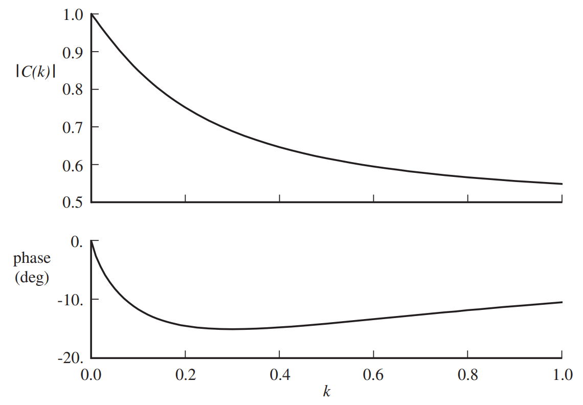
Theodorsen function $C(k)$ as a function of $k$ [source]
Aside
An alternate form of looking at \(C(k)\) is that it is a transfer function of the linear fluid system, since fluid has been modelled using potential flow theory which is based on the linear Laplace’s equation, such that when the input to the system is the motion the final output is a response at the same frequency but with a phase delay and change in amplitude.
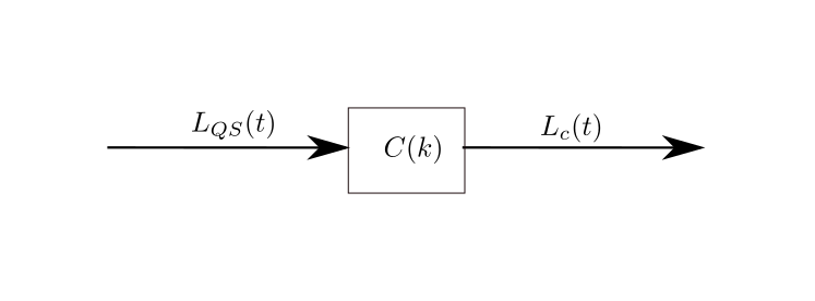
Theodorsen function as a response transfer function
For an exemplary case of an airfoil of chord \(c\) pitching as \(\alpha = \alpha_0 \sin (\omega t)\) in an oncoming flow with freestream velocity of \(U_\infty\), the corresponding unsteady lift then is given by
where \(\phi\) is the phase of the complex \(C(k)\) at \(k=\omega b/U_\infty\).
Summary and Final Thoughts
In summary, unsteadiness comes from accounting for the vorticity in the wake and when wake vorticity (as in the case of the starting vortex) is not acocunted for the flow is considered to be steady. In addition, a steady airfoil generates lift which is purely due to the circulation of the flow but an airfoil undergoing unsteady motion will generate an added lift that is due to the displacement of the surrounding fluid.
The Theodorsen model is a solution of the unsteady potential flow so the problem of fluid flow represents a linear problem. Potential flow theory is based on the inviscid assumption so clearly the predicted drag force (i.e. force along the direction of flow) is zero leading to the d’Alembert’s paradox. Of course this is not much of a paradox now given we modelled the fluid as an ideal fluid is some sense by ignoring viscosity altogether. Therefore, the Theodorsen model does not make any prediction about the nature of drag.
From the discussion till now, it is clear that there is a significant difference between the wake of an airfoil when it maintains a constant angle of attack versus when the airfoil is pitching. The difference arises due to the shed vorticity in the airfoil wake. In case of steady airfoil, the starting vortex convects far away but in case of the pitching airfoil vorticity is constantly being shed due to the changing bound circulation around the airfoil. These shed vortices in the vicinity of the airfoil have the potential to influence the aerodynamics of the airfoil and need to be accounted for. The criterion used to decide the threshold when unsteady aerodynamic effects might be significant enough, that they cannot be ignored, is called reduced frequency.
Finally, in general, in order to evaluate the aerodynamic load (steady or unsteady) acting on rotating wings, the set of non-linear PDE called NSE need to be solved. This can be a daunting excercise using CFD methods that is both computationally intensive, i.e. requiring significant computing infrastructure, as well as time consuming, i.e. it would be a few days before you would see the final result! The lifting line theory presents a great simplification in that what happens to the flow in the rotor wake can be modelled separate from the effect of flow on the blade itself. The effect of the rotor wake is modelled as an inflow that can be obtained via a hierarchy of inflow models of varying levels of fidelity but we discussed the simplest ones in this course - the momentum theory and the blade element momentum theory. The blade element momentum theory requires prior knowledge of the airfoil characterisicts (i.e. \(C_l\), \(C_d\) and \(C_m\)) but presents a vast improvement over the simple momentum theory in that the effect of using different airfoils making up the blade sections can be accounted for. These airfoil characteristics are based on steady state airfoil aerodynamics. This solution strategy has proven to provide acceptable results in hover and very low speed forward flight but not for high speed forward flight cases.
When unsteady motion of the airfoil is involved, like in forward flight conditions, even an airfoil has a wake whose effect on the airfoil section itself needs to be accounted for in order to evaluate lift, drag and moment on the airfoil accurately. So if we consider the general case of a rotor where the blades are undergoing unsteady motion then one component of the rotor wake vorticity is due to the finiteness of the wings and a secondary component now exists due to the unsteady motion of the blade sections that make up the rotor. Instead of solving for the influence of this combined complex wake on the blade sections, i.e. evaluating the induced inflow, we use the same strategy as used in the case of steady rotor aerodynamics. We can do this be evaluating the effect of the unsteady airfoil wake on the airfoil loads, this is where the Theodorsen theory comes in handy when harmonic motion is involved. Once the effect of the airfoil wake has been accounted for, the effect of the rest of the wake (due to finite wing effects) can be treated using blade element momentum theory. This is the standard process used for modelling rotor aerodynamics using ‘non-CFD’ methods. There exist a number of unsteady airfoil aerodynamics analysis models (particularly in the field of helicopter aerodynamics) one can choose from - Peters model, indicial response methods, state-space modelling etc. - for quantifying the airfoil wake effects on blade section loads and once they are known the rotor inflow can be obtained using BEMT. Here too a number of models exist in addition to the annular momentum theory - for e.g. dynamic inflow, free-wake, lifting surface, vortex particles etc.- but, irrespective of the specific models used, the overarching strategy towards a quick solution follows the standard strategy convexed through this course.