Forward Flight
Contents
Forward Flight
“The problem of the rotor in steady forward flight is the problem of defining the magnitude and direction of airflow encountered by each blade element”
—Alfred Gessow (Aerodynamics of the Helicopter)
Discussing about the details of forward flight state aerodynamics is also the perfect time to talk about the 2D aerodynamic characteristics of the airfoil sections that make up the blades of the rotor. You would not be prepostrously wrong in assuming that if the blade sections are made up of an airfoil with better airfoil characteristics then the overall rotor efficiency would be improved. ‘Efficiency’ of the rotor here refers to just the profile + induced power consumption of the rotor but in literature this term can also be used to refer to the acoustic noise or vibratory characteristics of the rotor. These are not within the scope of this course so we’ll just end up focussing on rotor power consumption. But what does ‘better airfoil characteristics’ precisely mean? Is it just larger \(C_l/C_d\)? Larger stall angle of attack? The way the question has been posed might suggest that indeed there is something extra that needs to be accounted for or considered in order to improve rotor performance in forward flight. What that ‘extra’ might be would become clear as the various aerodynamic phenomena, encountered by the rotor, in forward helicopter flight are discussed.
On a conventional helicopter, the rotor is the sole entity responsible for generating thrust to counter the weight as well as the fuselage drag. While this characteristic itself leads to interesting aerodynamics and rotor performance attributes, there are a ton of pecularities arising just from edgewise rotor flight.
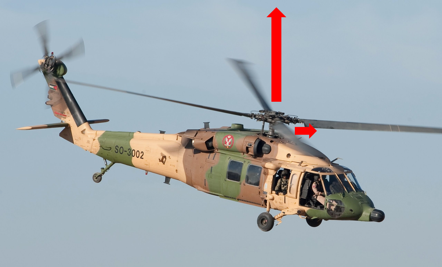
UH-60A Helicopter [source]
Fixed-wing wake vs Rotary-wing wake
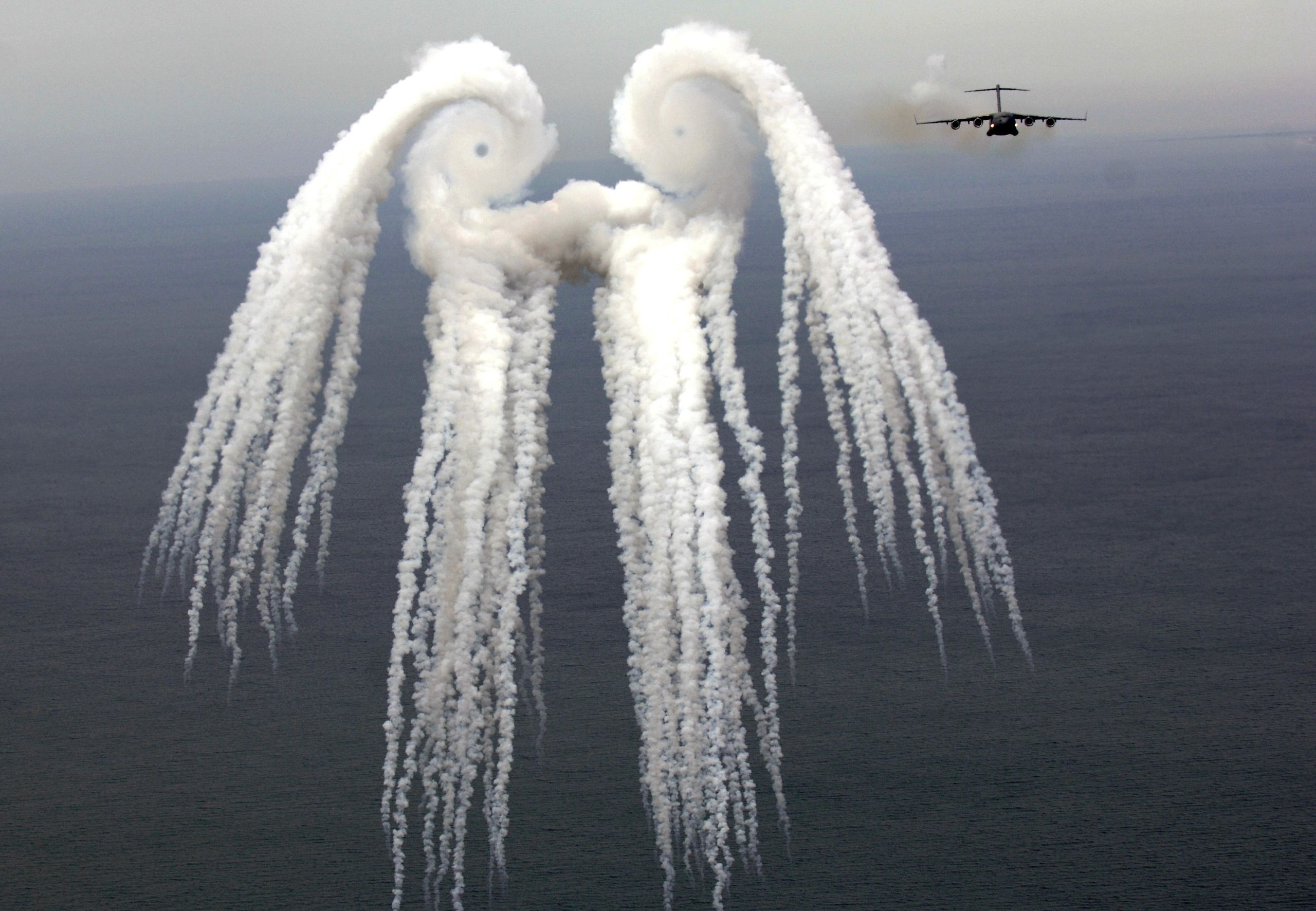
Wing tip vortices behind a Boeing C-17 Globemaster [source]
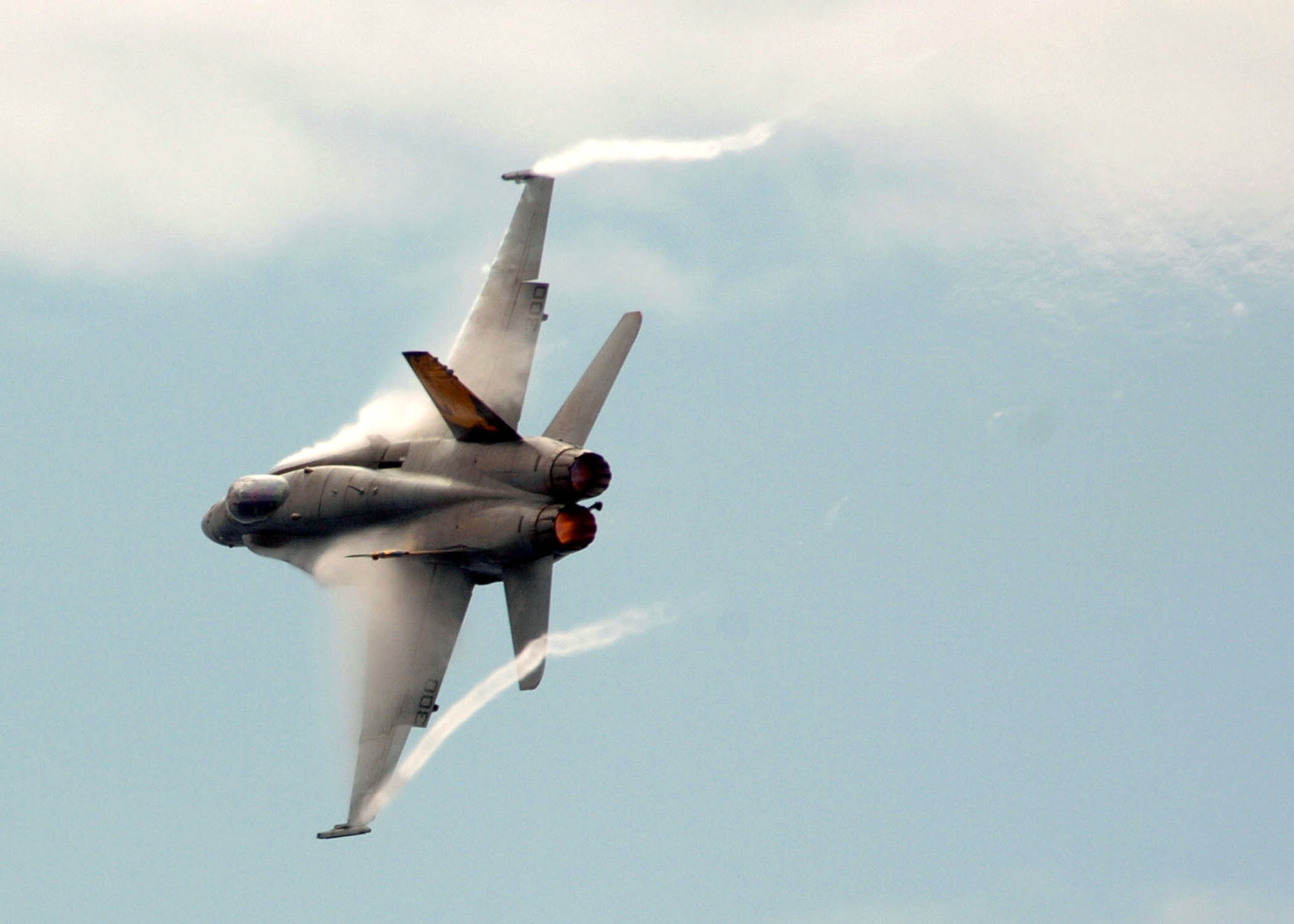
Wing tip vortices behind a McDonnell Douglas F/A-18 Hornet [source]
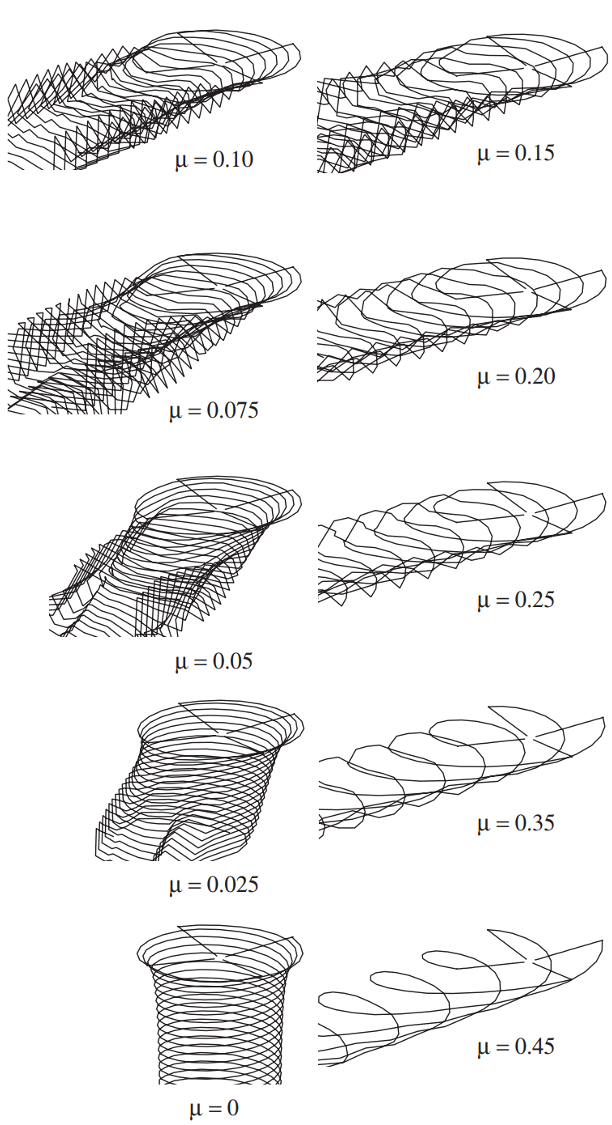
Rotor tip vortex trajectories at difference advance ratios [source]
Note the changing wake pattern with \(\mu\)
\(v_i\) due to vortex-induced velocity
Biot-Savart law
high \(v_i\) with tightly spaced rings in hover
high induced power
low \(v_i\) when rotor quickly moves away
low induced power
fast forward flight
rotor in climb
vortex-based methods for better accuracy
free-wake
CFD
Free-wake simulation of a 4 bladed rotor in forward flight
from IPython.display import YouTubeVideo
YouTubeVideo('7PcowKB_Dwc', start=0, end=40, width=750, height=400)
Induced power
The induced velocity in forward flight is stated below. It is to be assumed as agiven. It can be derived using the same principles that the expression for hover and climb cases were obtained, and is again based on the uniform inflow velocity assumption.
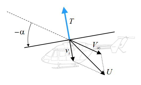
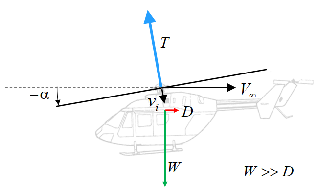
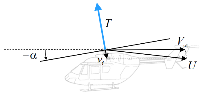
where \(U = \left | \bar{V_{\infty}} + \bar{v_i} \right |\) is the vector sum of the oncoming flow velocity and the induced flow velocity. This result is consistent with the expressions obtained for hover and axial flight in that it reduces to the corresponding expressions when appropriate substitutions are made for \(U\) and this is shown below. The induced power is then simply given by \(P_i=Tv_i\). Note that \(\alpha\) in the proceeding results refers to the shaft tilt angle from the vertical position (and not angle of attack) which by convention is taken as positive for a rearward rotor disk tilt.
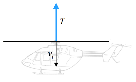
Hover
Vertical climb
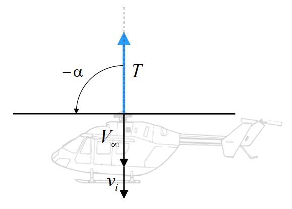
Low forward speed
The low forward speed assumption of \(\alpha\approx 0\) is generally valid for advance ratios \(\mu<0.15\), where \(\mu = \frac{V_{\infty}}{\Omega R}\).
High forward speed
![[source]](https://en.wikipedia.org/wiki/Sikorsky_UH-60_Black_Hawk#/media/File:Jordanian_Air_Force_UH-60_Black_Hawk_helicopter_(cropped).jpg)
![[source]](https://en.wikipedia.org/wiki/Wingtip_vortices#/media/File:C17-Vortex.JPG)
![[source]](https://en.wikipedia.org/wiki/Wingtip_vortices#/media/File:FA-18C_vapor_LEX_and_wingtip_1.jpg)
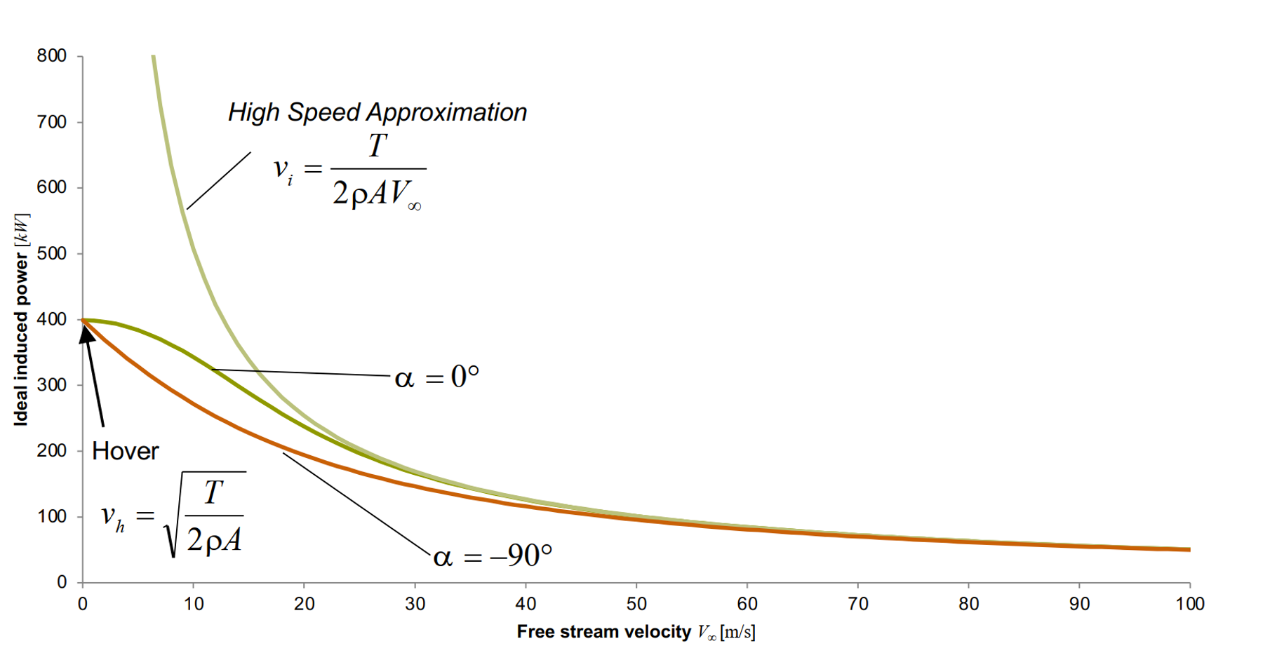
The inflow variation with forward speed can then be obtained by stitching-up the results in the different domains. Once the induced velocity is known, the induced power can be simply obtained as \(Tv_i\). As was mentioned earlier for hover, large mass flow through the rotor disk is key to thrust efficiency of a rotor. When a rotor is tilted for forward flight, a component of the oncoming flow velocity goes through the rotor disk. This increases the effective mass flow rate of air through the disk much like in the rotor climb scenario. Consequently, a smaller increase in velocity needs to be imparted to the flow to get the required momentum change and leads to the reduction in \(v_i\) obtained.
Descent flight
Descent flight in rotorcraft is usually undertaken at very low speeds. Fast descent speeds can lead to large flow recirculation and turbulence in the flow, leading to high vibrations and loss of control. There are three distinct states that exist with increasing descent flight velocities of a rotor -
Vortex ring state
\(V<0\) but \(V+v_i>0\)
Turbulent wake state
\(V<0\) and \(V+v_i<0\), but \(V+2v_i>0\)
Windmill brake state
\(V<0\), \(V+v_i<0\), \(V+2v_i<0\)
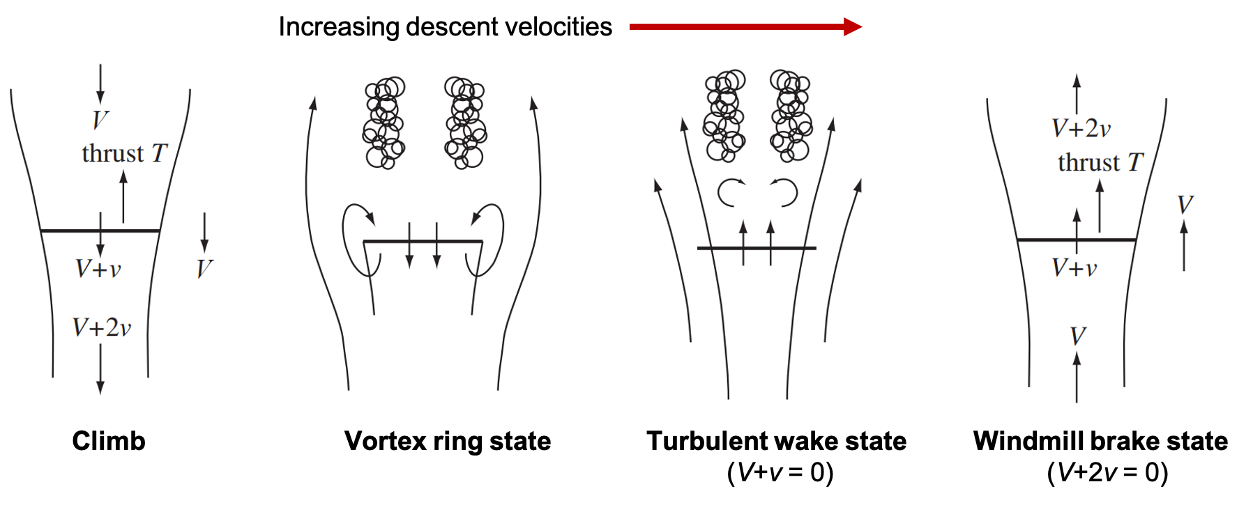
Rotor descent flight states [source]
from IPython.display import YouTubeVideo
YouTubeVideo('HjeRSDsy-nE', width=750, height=400,start=133)
from IPython.display import YouTubeVideo
YouTubeVideo('05_WFvh9ISk', width=750, height=400)
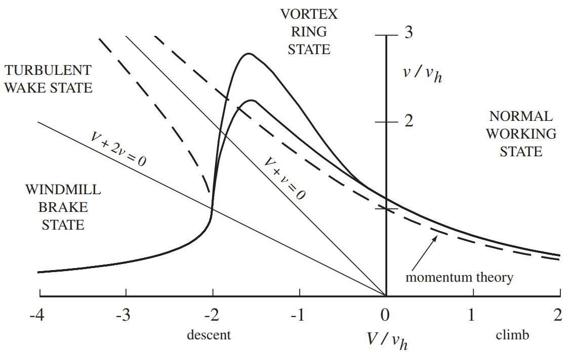
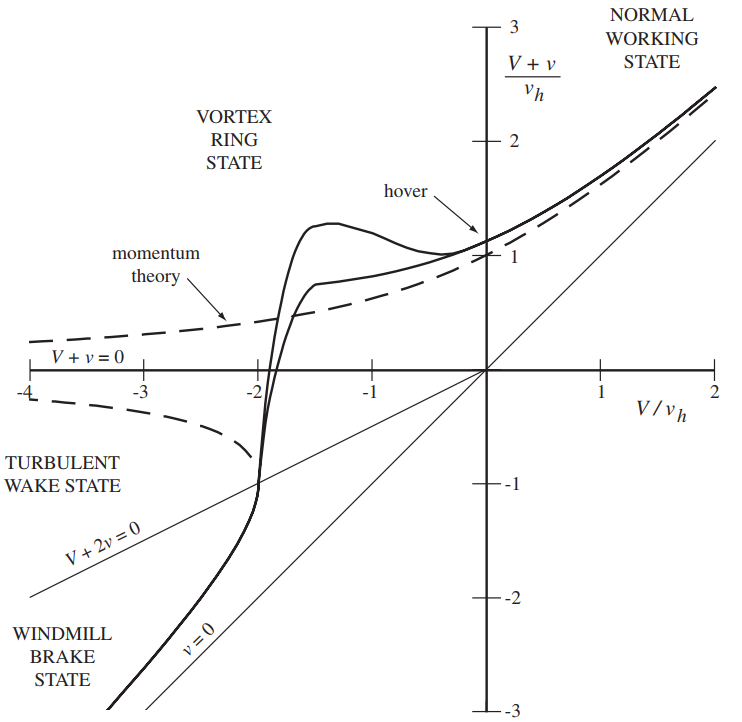
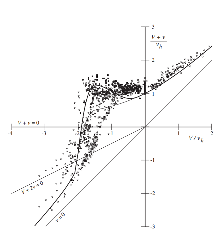
The following show induced velocity of the rotor as a function of climb velocity (negative climb velocity denotes a descent flight state). While not explicitly derived as part of the lectures, the inflow velocity during the windmill brake state, i.e. when the rotor acts as a wind turbine, can be derived using momentum theory along the lines of the derivation for the normal working state. The variation would then be as denoted by the solid lines. However, if the results were simply extended (denoted using dashed lines) to regions that we now understand to be the turbulent wake state or the vortex ring state, the results would not match with that observed in reality (solid lines). This is because the flow is highly turbulent in these scenarios and the simple momentum theory does not capture that and incurs an error. An alternate way of presenting the same results is by plotting the total inflow velocity on the y-axis. When experimental measurements are laid on this figure, notwithstanding the scatter in the measurements, they largely follow the trend of the solid lines.
It is worth noting that these experimental results are not based on a measured induced velocity in wind tunnel or free-flight, rather the total power consumption of the rotor was measured and simple momentum theory-like relations were assumed to arrive at the corresponding uniform induced inflow velocity. This is why the second plot of total inflow versus climb velocity is used because the total power measured in experiments can be directly used to obtain the net inflow since climb power and induced power cannot be separately measured. Another feature apparent from the figures is that momentum theory, as simple as it is, is capable of predicting the average rotor power consumption very well.
Note that convention followed within these figures is such that \(v\) is used to represent inflow velocity \(v_i\), \(V\) is used to denote climb velocity \(V_c\), and \(v_h\) refers to the induced velocity at hover.
Rotor aerodynamics assymetry
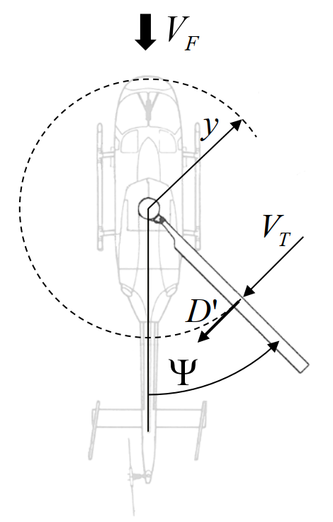
As soon as a rotor starts moving edgewise, a lateral assymetry is introduced with regard to the total in-plane velocity. This assymetry is most prominent at the azimuth locations \(\psi=90°\) and \(\psi=270°\) and decreases progressively to no assymetry at azimuth locations \(\psi=0°\) and \(\psi=180°\).
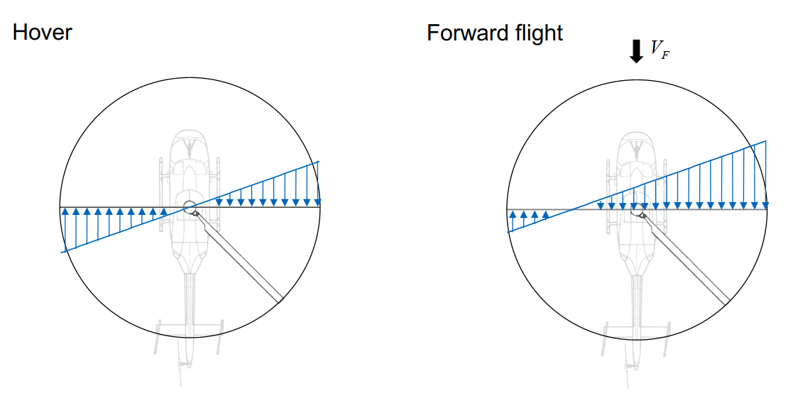
Tangential velocity distribution in hover versus forward flight (at $\psi$ =90°)
Reverse flow
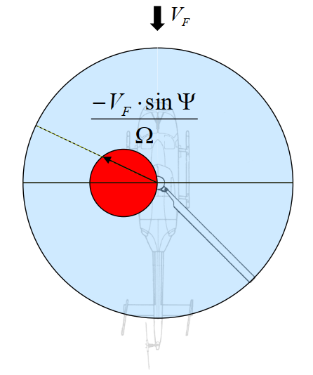
Along with the in-plane flow assymetry in the lateral direction, a reverse flow region occurs in forward flight. This is of concern because the blade sections within this region effectively have an angle of attack close to 180° and are no longer aerodynamically efficient. There is no minimum threshold speed for the reverse flow region to occur but it is not of major concern for low speed flight since rotors generally have a root cutout region of about 20%. Based on the equations given below, this means that only for \(\mu > 0.2\) do blade airfoil sections start experiencing reverse flow.
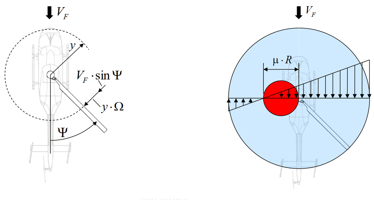
Reverse flow region during forward flight
Profile power
The drag due to fluid viscosity and due to pressure distribution over the airfoil surface manifests itself within the airfoil drag coefficient. The power required by the rotor to overcome these drag forces can be evaluated by integrating the power required to overcome drag at each blade section and averaged over the azimuth.
Blade section drag due to in-plane velocity
Rotor in forward flight
Parasite power
The power expended in order to overcome the fuselage drag of a helicopter is refered to as the parasite power. It is simply the parasite drag times the forward speed where the parasite drag itself is usually stated as an equivalent flat plate area \(f\). Since fuselage attitude largely remains the same at any speed, \(f\) can be assumed a constant.
Power bucket curve
The consumed power breakdown of the entire helicopter is shown below. The power required by the tail rotor \(P_{TR}\) which can be fairly approximated as a fixed percentage (about 10%) of the total power required by the main rotor 1. \(P_a\) here refers to accesories power for onboard equipment and \(P_{tl}\) refers to additional power required to overcome transmission losses. These three power components are small in comparision of the main rotor power \(P_i+P_0\) and the helicopter parasite power \(P_p\). The characteristic ‘bucket’ curve is a byproduct of the interplay between the latter 3 power components.
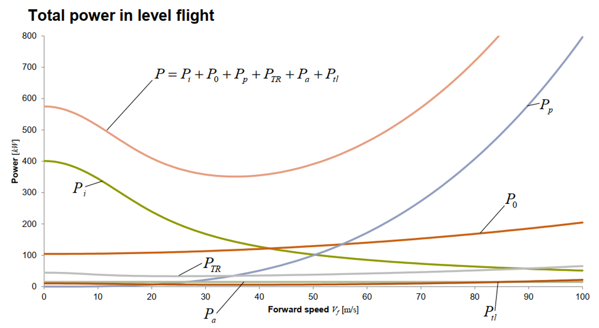
Total helicopter power consumption versus forward speed
- 1
Alternately, the tail rotor power can be also obtained from first principles using BET or momentum theory.