Blade element momentum theory¶

From the momentum theory analysis, the following relations were obtained relating rate of mass flow of fluid (air) through the rotor disk, the thrust generated, and the corresponding power required.

\[T=\dot{m} w=2\rho A v_i^{2}\]

\[P=\frac{1}{2} \dot{m} w^{2}=2 \rho A v_{i}^{3}\]

Annular momentum theory¶

It was assumed that the inflow velocity \(v_i\) was uniform over the entire rotor disk. In reality that is not true. However, instead of analysing the more general case where \(v_i = f(r,\psi)\), where \(\psi\) is the azimuth or polar angle over the rotor disk, we continue working with the axial flight scenario where \(v_i\) is some function of only \(r\) (i.e. an azimuthal symmetry exists). In order to arrive at the thrust and power relations like above, the rotor disk is discretised into rings and elemental thrust contribution from each ring is calculated. The overall rotor thrust is then just an integrated quantity.

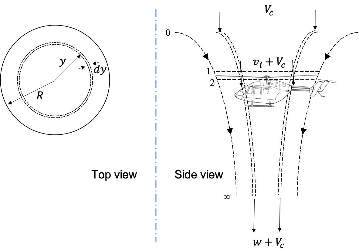
Annular momentum theory model

(4)¶\[\begin{align} d T & =wd \dot{m} \\ &= 2v_{i} \rho 2 \pi y d y\left(V_{c}+v_{i}\right) \\ d C_{T} & =\frac{4 \pi \rho\left(V_{c}+v_{i}\right) v_{i} y d y}{\rho \pi R^{2}(\Omega R)^{2}}\\ &=4 \lambda \lambda_{i} r dr \\ &=4 \lambda \left(\lambda-\lambda_{c}\right)r d r \\ C_{T} &= 4 \int \lambda \left(\lambda-\lambda_{c}\right) r d r \quad \quad \text{Climb case}\\ &= 4 \int \lambda^{2} r d r \quad \quad \quad \quad \quad \text{Hover case} \end{align}\]

where, the inflow ratio \(\lambda = (V_c+v_i)/\Omega R\) 1, \(\lambda_i = (v_i)/\Omega R\) and \(\lambda_c = (v_c)/\Omega R\)

The expressions obtained above relate rotor thrust in case the inflow velocity is a function of radial location. This is a massive improvement from the uniform inflow case but we would still like it if the model incorporated airfoil aerodynamics in some way. Recall that a similar relation was obtained for the thrust coefficient using BET but, in lieu of being able to quantify the inflow velocity more appropriately, simply the uniform inflow momentum theory result was used. Marrying the two give us the blade element momentum theory (BEMT).

Blade element momentum theory (BEMT)¶

From BET: \( \displaystyle \quad d C_{T}=\frac{\sigma}{2} C_{l_{\alpha}}\left(\theta r^{2}-\lambda r\right) d r\)

From annular momentum theory : \(\displaystyle \quad d C_{T}=4 \lambda\left(\lambda-\lambda_{c}\right)rd r\)

\[\Rightarrow\displaystyle d C_{T}=\frac{\sigma}{2} C_{l_{\alpha}}\left(\theta r^{2}-\lambda r \right) d r =4 \lambda\left(\lambda-\lambda_{c}\right)rd r\]

\[\displaystyle \Rightarrow \frac{\sigma C_{l_{\alpha}} \theta r}{8}-\frac{\sigma C_{l_{\alpha}}}{8} \lambda=\lambda^{2}-\lambda_{c} \lambda\]

\[\displaystyle \Rightarrow \lambda^{2}+\left(\frac{\sigma C_{l_{\alpha}}}{8}-\lambda_{c}\right) \lambda-\frac{\sigma C_{l_{\alpha}} \theta r}{8}=0\]

\[ \lambda\left(r\right)= \displaystyle \pm \sqrt{\frac{\left(\frac{\sigma C_{l_{\alpha}}}{8}-\lambda_c \right)^2+\frac{\sigma C_{l_{\alpha}} \theta r}{2}}{4}} - \displaystyle \frac{ \frac{\sigma C_{l_{\alpha}}}{8}- \lambda_c}{2} \]

Much like the momentum theory analysis of a climbing rotor, here again the negative root is ignored because it does not comply with the physical system we assumed in the beginning i.e. flow velocity at every cross-section of the stream tube is downwards. Further, if just the hover inflow velocity is concerned, the following expression can be derived:

\[\begin{equation*} \begin{split} \lambda (r)=\frac{\sigma C_{l_{\alpha}}}{16}\left[-1+\sqrt{1+\frac{32}{\sigma C_{l_{\alpha}}} \theta r}\right],\quad\quad\quad \text{for} \quad\lambda_c=0 \end{split} \label{eq:BEMT_lambda} \tag{2} \end{equation*}\]

Eq \(\eqref{eq:BEMT_lambda}\) is one of the most useful results one can obtain in so far as the amount of effort required in understanding the origins of that result as well the ease of analysing real rotors with it is concerned. This expression takes into account the following - blade geometry via \(\sigma\), airfoil aerodynamics via \(C_{l_{\alpha}}\) and blade twist distribution via \(\theta\). After obtaining \(\lambda(r)\), \(C_T\) can be obtained by just substituting back in \(C_T = \int 4 \lambda (\lambda - \lambda_c)rdr \) (or should you use the BET expression \( \displaystyle \quad d C_{T}=\frac{\sigma}{2} C_{l_{\alpha}}\left(\theta r^{2}-\lambda r\right) d r\) ?).

Is there something that you can think of that Eq. \(\eqref{eq:BEMT_lambda}\) doesn’t model/account for?

Airfoils are a 2D entity whose aerodynamic characteristics provide us with basic building blocks for modelling overall aerodynamics of real 3D wings (the technical term usually used to refer to the 3D wing aerodynamics is finite-wing aerodynamics). In reality aerodynamics are always 3D, atleast in the context of flying vehicles. Turns out the situation in 3D is not a straightforward conglomeration of the 2D section aerodynamics. There are additional effects that occur in real flows over wings which do not occur when the flow is assumed to be 2D. Not accounting for these 3D effects, depending on how potent they are compared to the 2D aerodynamics, can lead to inaccurate results. So, while the Eq \(\eqref{eq:BEMT_lambda}\) is useful for all the reasons given earlier, it doesn’t model everything. For example, the effects of blade spanwise radial flow, unsteady aerodynamics, dynamic stall, additional vortex roll-ups are not accounted for.

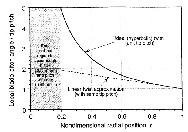
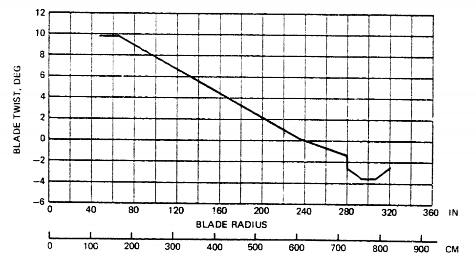
Ideal twist¶

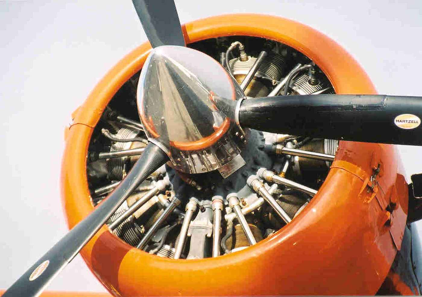
Propeller [source]

Based on the inflow relation in Eq \(\eqref{eq:BEMT_lambda}\), it can be seen that \(\lambda(r)=\) const is obtained if \(\theta r =\) const. This twist distribution is refered to as hyperbolic twist and results in minimum induced power for a rotor (provided none of the other terms in Eq \(\eqref{eq:BEMT_lambda}\) change as a function of \(r\) of course). In reality, helicopter blades tend to have more or less a linear twist distribution of about -8° to -16° based on the span. While better hover performance is possible with even greater blade twist, it is detrimental to forward flight performance (leads to inboard sections stalling on retreating side) and so a compromise needs to be made. Propellers on the other hand are always in climb mode, which makes their operational environment to always have azimuthal symmetry (function of \(r\)), and are therefore highly twisted.

\[\lambda (r)=\frac{\sigma C_{l_{\alpha}}}{16}\left[-1+\sqrt{1+\frac{32}{\sigma C_{l_{\alpha}}} \theta r}\right]\]

Ideal blade twist distribution [source]

UH-60 rotor blade twist [source]

Optimum hovering rotor¶

From a theoretical point of view, a rotor design with a uniform distribution of inflow velocity over the rotor disk will lead to minimum induced power consumption. This is the power expended to impart kinetic energy to the flow in the rotor wake. Turns out, minimum work needs to be done by the rotor (and hence minimum induced power) when this flow velocity is constant over the disk. This can be proven using variational calculus but will not be taken up here. With the development of the BEMT principles above, we now look at what design requirements could the uniform inflow condition pose on the rotor geometry.

Recall from BET derivation:

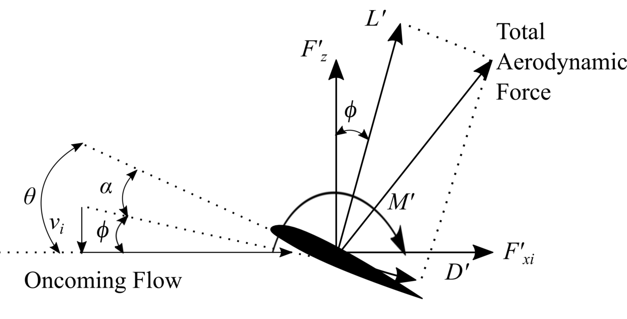
\[\begin{equation*} \begin{split} dC_T &= \frac{\sigma}{2} C_l {r}^2d{r} \\ &=\frac{\sigma}{2}C_{l_{\alpha}} \left(\frac{\theta_{tip}}{r} - \frac{\bar{\lambda}}{r}\right){r}^2 d{r} \\ \end{split} \label{eq:BEMT_idealtwist} \tag{3} \end{equation*}\]

where the ideal blade twist assumption has been made and \(\bar{\lambda}\) is the uniform inflow ratio and the angle of attack \(\alpha\) is given by,

\[ \alpha = \displaystyle \frac{\theta_{tip}-\bar{\lambda}}{r}= \displaystyle \frac{ \alpha_{tip}}{r}\]

So, the lift generated at a given blade section can be given by,

\[C_l = C_{l_{\alpha}} \frac{\alpha_{tip}}{r}\]

The overall rotor thrust, based on Eq \(\eqref{eq:BEMT_idealtwist}\), is then given by the expression

\[\Rightarrow C_T= \frac{\sigma}{4}C_{l_{\alpha}}\alpha_{tip}\]

So, within the scope of blade element momentum theory, a uniform induced velocity requires a hyperbolic blade twist which translates to a hyperbolic angle of attack distribution over the span of the blade. Even if it is not immediately obvious why such a design is not a practically feasible, it certainly sounds wrong - afterall hyperbolic twist is not realisable in practice. The more pertinent fact relates to the aerodynamics of airfoils, in that they don’t keep producing lift as the angle of attack is increased hyperbolically - they stall beyond an angle, called the static stall angle. However, given the way Eq \(\eqref{eq:BEMT_idealtwist}\) has been written down can be a recipe for confusion if one forgets that it is valid only in the linear regime of airfoil angle of attack. The presence of a root cut-out region on the rotor brings some relief, even if the hyperbolic profile is followed, because the angle of attack doesn’t need to keep increasing infinitely to realise uniform inflow towards the center of rotation.

Airfoils tend to exhibit best aerodynamic efficiency (i.e. generating highest lift for a unit amount of drag incurred) only at a certain \(\alpha\) for a given \(M\). So it seems desirable that all the blade sections should be operating at that value in order to minimise profile drag. Note that we have not discussed profile drag until now but it doesn’t take a stretch of the imagination to realise that the overall rotor would be most efficient if all blade sections were operating at \(\alpha\) for best \(L/D\) (henceforth refered to as \(\alpha_{L/D}\)). This angle varies slightly as a function of \(M\), so different blade sections would need to operate at slightly different \(\alpha_{L/D}\) in reality. We look at the geometric consequences of operating every blade section at \(\alpha_{L/D}\) and assume that it is independent of \(M\) and hence constant for all blade sections.

Recall from annular momentum theory:

\[\begin{equation*} \begin{split} d C_T = 4 \bar{{\lambda}}^2 r dr \end{split} \label{eq:MT_idealtwist} \tag{4} \end{equation*}\]

Comparing Eqs. \(\eqref{eq:BEMT_idealtwist}\) and \(\eqref{eq:MT_idealtwist}\), the corresponding (uniform) inflow ratio when the angle of attack is \(\bar{\alpha}_{L/D}\) over the span of the blade is given by:

\[\begin{equation*} \begin{split} \Rightarrow \bar{{\lambda}} = \displaystyle \sqrt{\frac{\sigma r C_{l_{\alpha}}\bar{\alpha}_{L/D}}{8}} \end{split} \label{eq:optimum_rotor} \tag{5} \end{equation*}\]

With all blade sections operating at constant \(\bar{\alpha}_{L/D}\), and uniform inflow over the entire rotor disk, from Eq. \(\eqref{eq:optimum_rotor}\) it is apparent that the rotor solidity would need to vary hyperbolically. This result is again not physically feasible but points to the benefits of introducing blade taper - i.e. progressively smaller chord outboard would help achieve best rotor performance based on the discussion so far.

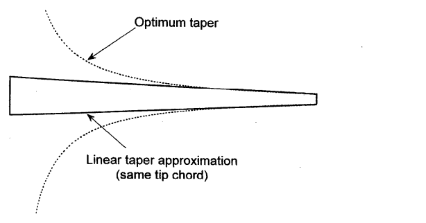
Optimum blade taper [source]

Profile power¶

The power consumption of a thrust-producing rotor in hover can be divided into induced power and profile power. The former has been discussed at length and is a result of the rotor imparting kinetic energy to the flow. The power expended to overcome drag due to viscosity of the flow is refered to as profile power and can be obtained in a straightforward manner following the same principles used to obtain induced power.

2D blade section aerodynamic loads

\[d F_{x}=d L \sin \phi+d D \cos \phi\]

\[d P= dP_i + dP_0=(\phi d L+d D) N \Omega y\]

\[d P_0=N \Omega y dD\]

\[d C_{P_0}=\frac{\sigma}{2} C_{d} r^{3} d r\]

Carrying out the above integration for the case of the optimum hovering rotor:

\[\Rightarrow C_{P_0} = \frac{1}{2} C_{d_{0}} \int {\frac{\sigma_{tip}r^3}{r}} d r=\frac{C_{d_{0}} \sigma_{tip}}{6}\]

Limitations¶

Modern manufacturing practices provide the flexibility of contructing blade with planforms that can potentially improve rotor efficiency - performance as well as acoustics. Given some of the optimised planforms that have been put into use recently (see below), the corresponding rotors cannot be analysed just using BEMT. This is because these rotors accrue performance benefits (power, acoustics, vibration) by predominantly exploiting 3D aerodynamic phenomena - such as blade vortex interaction (BVI), vortex roll-up, stall margin improvement etc. State-of-the-art rotors such as these are not a straightforward result of simply using airfoils that have shown improved 2D aerodynamic characteristics but an involved excercise of alleviating detrimental aerodynamic effects that are known to occur at the rotor level.

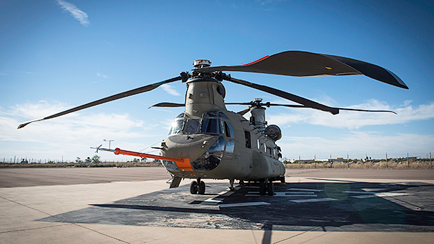
Advanced Chinook Rotor Blade (ACRB) [source]

Blue-Edge blade [source]

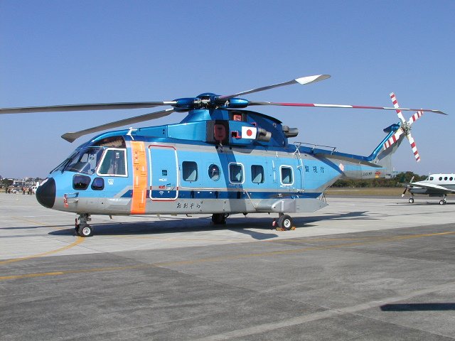
British Experimental Rotor Programme (BERP) blade [source]

from IPython.display import YouTubeVideo
YouTubeVideo('2t3uCDJhce8', width=700, height=300)

YouTubeVideo('OchreIBZknI', width=700, height=300)

The new Chinook rotor in action can be seen here [source]. Although, the ride was probably not a very smooth one [source].

Weighted Solidity¶

The rotor solidity is a geometric quantity defining the ratio of the total blade area by the area of the rotor disk. As seen already it comes up often in rotor analysis and holds information about a number of rotor geometric quantities together in one non-dimensional parameter. However, solidity can also be defined locally……. The idea comes from a need for comparing two rotor designs that have different planform shapes2.

\[\sigma_{rotor} = \frac{\text {blade area}}{\text {rotor area}} =\int_{0}^{1}\sigma dr \]

The thrust-weighted solidity, as the name implies, is the fictional solidity of the rotor obtained by weighting the solidity at a particular section with the corresponding thrust generated. A rotor with a larger lifting area on the outboard sections (for e.g. BERP rotor) can, in principle, be more efficient than a rotor with rectangular blades for the same overall solidity. This is because the former has larger lifting surface in the outer region where high dynamic pressure can help generate more thrust. A naive comparision might at equal solidities of the two rotors may not entirely be fair. In such a scenario, if the rotors are being compared at the same thrust setting then the thrust-weighted solidity of the rotors needs to be matched for a fair comparison.

\[C_T=\frac{1}{2}\int_{0}^{1}\sigma C_l r^2 dr = \frac{\sigma_e}{2}\int_{0}^{1} C_l r^2 dr\]

\[\Rightarrow \sigma_e=\frac{\frac{1}{2}\int_{0}^{1}\sigma \bar{C_l} r^2 dr}{\frac{1}{2}\int_{0}^{1} \bar{C_l} r^2 dr} = 3\int_{0}^{1}\sigma r^2 dr\]

\(\sigma_e\) here is the thrust-weighted solidity for the case of a uniform \(C_l\) rotor. Alternately, if the rotors are being compared at the same power setting then the power-weighted solidity is also used as a basis for comparing different rotor designs.

\[ \sigma_e=\frac{\frac{1}{2}\int_{0}^{1}\sigma C_{d0} r^3 dr}{\frac{1}{2}\int_{0}^{1} C_{d0} r^3 dr} = 4\int_{0}^{1}\sigma r^2 dr\]

This definition is also relevant because \(C_T / \sigma\) is used as a measure of the lifting capability of the rotor since it is nothing but the average lift coefficient of the blade sections.

\[\frac{C_T}{\sigma_e}= \frac{\bar{C_l}}{6}\]

\[ \frac{C_T}{\sigma_e}\vert_{max} \approx 0.15\]

The rotor \(C_T\) in forward flight is limited by the lifting ability of the blades when they are on the retreating side. High \(\sigma_e\) will ensure larger blade area contributes to rotor thrust on the retreating side so angles of attack on retreating side can be made lower (for same \(C_T\)). This will become clearer when forward flight has been discussed.

Summary and conclusion¶

Simplest strategy of separating blades aerodynamics and inflow
Higher-fidelity solution strategies employ same principle!
Different rotor wake (to evaluate \(v_i(r,\psi\))) exist
- high-fidelity analyses using CFD methods
- vortex particle methods [SF18]
- dynamic inflow models [Ban20, He89, Mur08]
- prescribed wake methods

1: in a past lecture, \(\lambda = v_i/\Omega R\) was stated for hover case. In general, it is the ratio of the total flow velocity at the rotor disk and the blade tip speed.
2: Comparing two rotors using this concept only works when the designs are not significantly different from rectangular blades. Because different aerodynamic effects come into play otherwise and this simple concept seizes to be useful.

Fundamentals of Helicopter Aerodynamics

Blade element momentum theory

Contents