Blade element theory
Contents
Blade element theory
“Remember that all models are wrong; the practical question is how wrong do they have to be to not be useful.”
Despite all the simplifications involved in the theoretical framework involving momentum theory, all the reasons why it is relevant were laid out in an earlier lecture. This was the only theory known for rotor analysis around the time VTOL inventions were taking-off (pun intended). So, for what its worth, initial helicopter rotor designs were surely dictated in some manner by analyses based on momentum theory. One major drawback that has been stressed upon is the lack of any direct relation between rotor aerodynamics and blade sectional aerodynamics. The Blade Element Theory (BET) takes care of that by incorporating airfoil aerodynamics. Therefore, unlike momentum theory which only has radius as the design variable, BET can be used in a more detailed design of the rotor. The central idea is that rotors are made up of blades (or wings) whose cross-sections are shaped like airfoils. The integrated effect of discretized sections of the blades leads to all the rotor forces and moments experienced at the rotor hub. In the following, the airfoil aerodynamics are accounted for but certain simplfying assumptions still persist lest things get hopelessly complicated. In general, BET refers to a whole class of modelling frameworks where the inflow velocity at the rotor disk is evaluated using a separate model - ranging from simple momentum theory to vortex-based models - while the blade aerodynamics is evaluated using blade 2D section (airfoil) aerodynamics.
The spacing between rotor blades is generally large enough that there is no blade-blade interference except perhaps in the case of co-axial rotors where the rotors are stacked close to each other. There is another form of blade-blade interference that exists in the form of interaction of the wake of the blades. This is referred to as BVI and in helicopter rotors this occurs during low speed flight when the rotor disk has a low negative tilt or positive tilt angle. When none of the aforementioned intereference effects occur, the rotor blade can be modelled as an independent entity and simply the sum of the time-varying forces on each blade can be added together to give the rotor forces over time. One can go a step further and model the blade itself as being composed of number of airfoil sections. That way the blade lift and drag, and by extension rotor thrust and torque, can be evaluated as function of airfoil aerodynamic characteristics and the local flow angle of attack at each section. That is precisely the premise of this chapter and the next. Note that the fundamental assumption here is that each blade section operates independent of all other blade sections. This assumption is not entirely acceptable for rotors because in certain positions over the rotor azimuth substantial radial flow can occur over the blade span, influencing the section boundary layers and the aerodynamics at any given blade section. However, radial flow corrections can be carried along the lines of sweep corrections in fixed-wing analysis [Joh13](Section 6.22) and will not be further discussed here. Additionally, when blade-blade interactions do occur and absolutely need to be accounted for, the underlying rotor analysis is still be based on BET or BEMT and additional vortex-based modelling strategies can be incorporated to account for such effects. All in all, BET is a powerful rotor modelling framework that combined with a judicious application of correction strategies can lead to very accurate results. In fact, this solution strategy forms the basis of rotorcraft analysis models commonly referred to as ‘comprehensive analysis’ within the community.
Disclaimer
Helicopter blades are flexible structures generally classified as beams due to their slender nature i.e. their length or span is quite larger compared to their width or chord. Thrust producing rotors of any kind are basically cantilevered beams so they undergo quite a bit elastic deformation. In case of helicopters, edgewise or forward flight of the rotor introduces periodic loading on the blades. Early rotor designs used blades made out of metal but current designs almost are constructed using composite materials due to their better fatigue properties [Hod06](Chapter 1, Pg 2). Whenever elastic aerodynamic structures are involved, there can be no standalone structural analysis or standalone aerodynamic analysis that would lead to a accurate result. The aerodynamic loading affects the structural deformation and that in turn influences the aerodynamic loads. This is a classic fluid-structure interaction problem that is encountered on helicopter rotors. That said, the trends in rotor performance can usually be captured very well assuming rigid rotor blades as well as provide insight into the phenomenology of rotor physics.
Mathematical formulation
Now that rotor parameters (beyond just radius) can be accounted for using BET, the following definitions come in handy -
Inflow ratio
Non-dimensional radial location
Solidity of the rotor
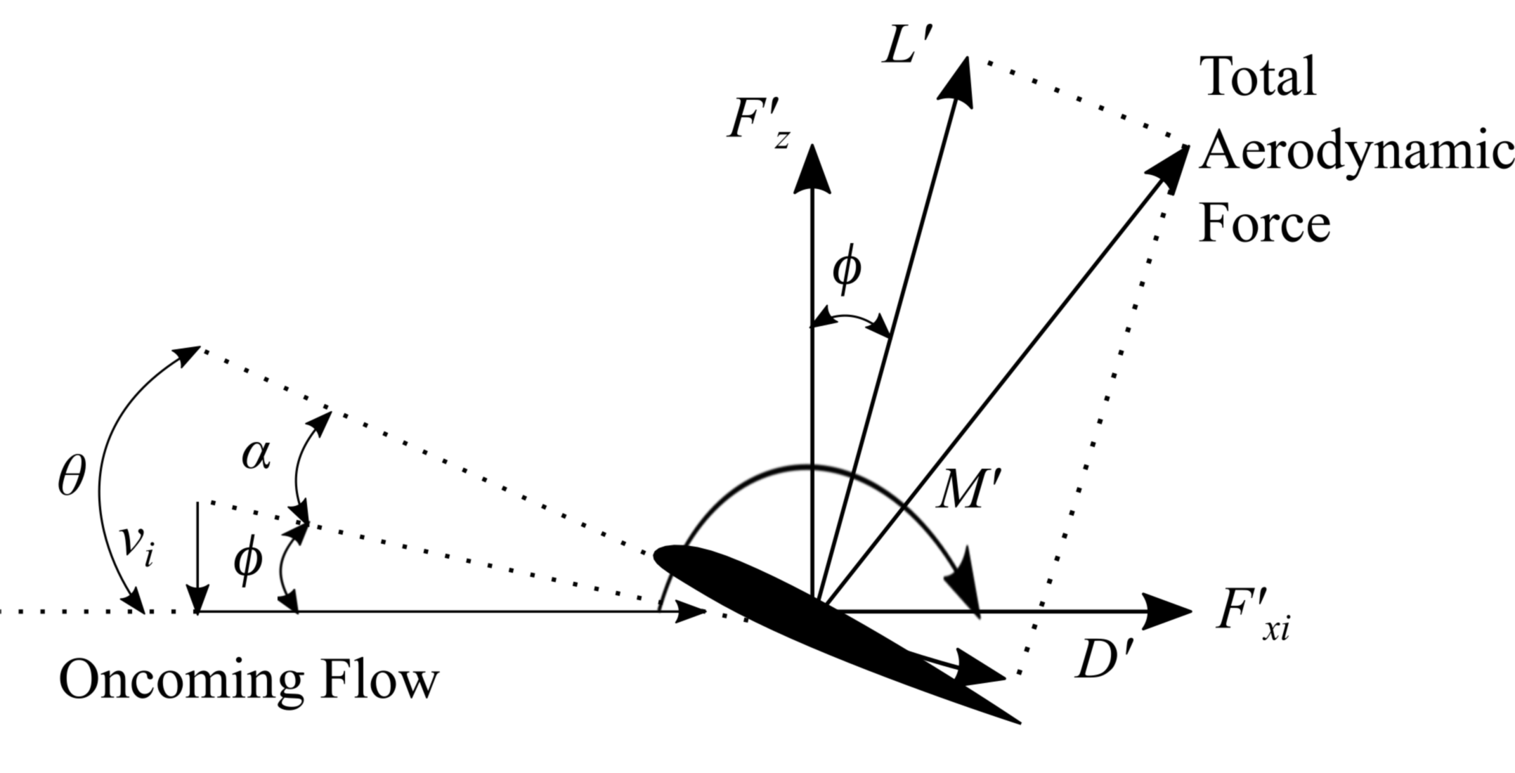
Note that the lift and drag vectors shown in schematics are not scaled for clarity of representation. In reality, an airfoil exhibits lift/drag of upto 80 and a more accurate vectorial representation of airfoil lift and drag is given by the following schematic
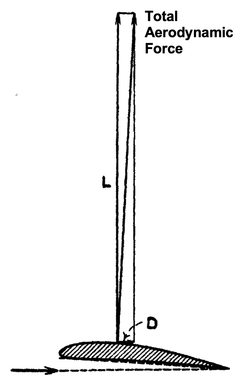
Representative aerodynamic lift and drag on an airfoil (modified from [source])
Assuming that the airfoil operates within the range where \(C_l\) varies linearly with \(\alpha\), the thrust coefficient contribution due to the blade elements can be integrated and written as
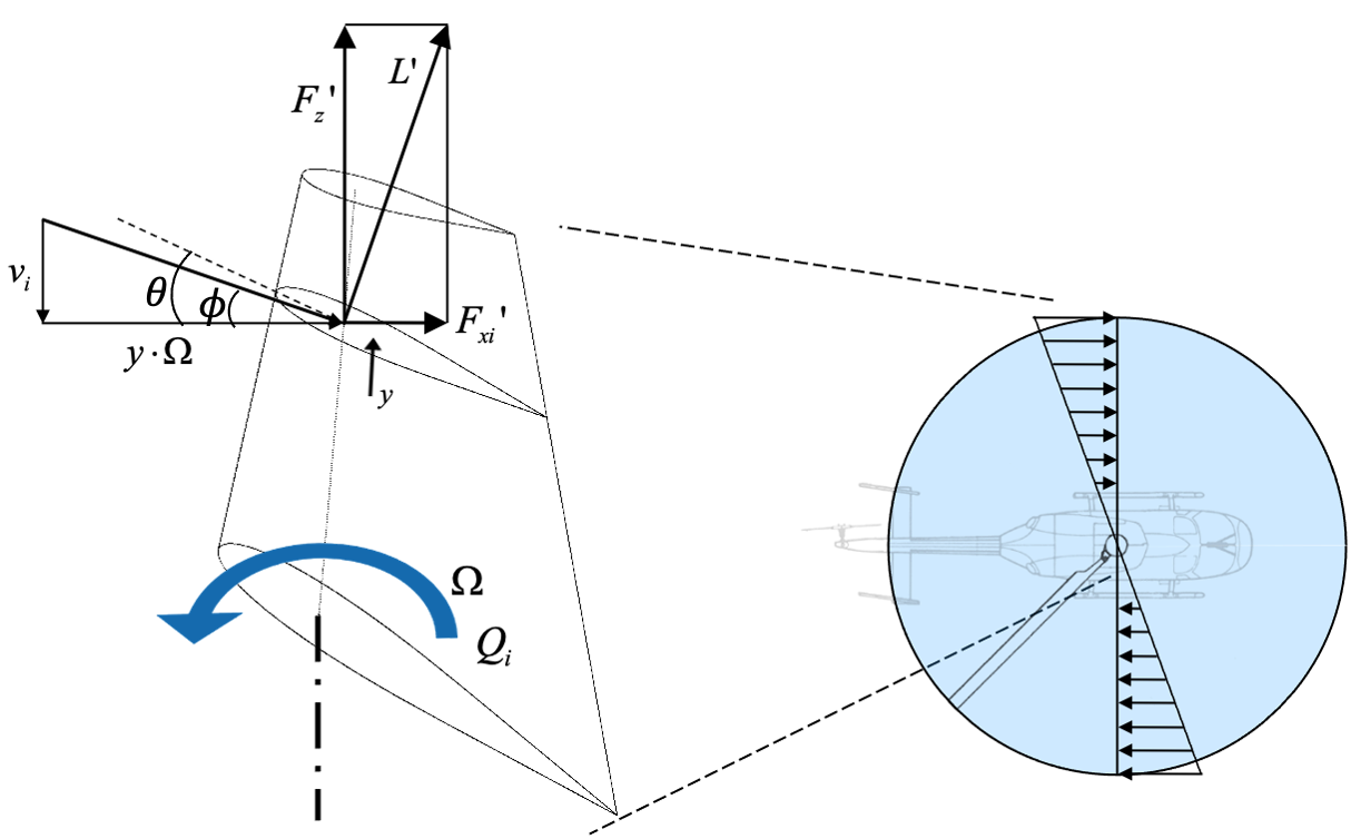
where \(U_P\) is the flow velocity perpendicular to the rotor disk (which in the case of hover is simply \(v_i\)) and \(U_T\) is the tangential flow velocity in the plane of the rotor disk.
In case of untwisted blades and uniform inflow, \(\theta\) and \(\lambda\) are constants. This is a highly restrictive assumption and one that is not found on real-world VTOL aircraft. Blades on all rotors have some built-in twist, this includes aircraft propellers, helicopter rotors, wind turbines etc. Slender rotor blades, as seen on full-scale helicopters or on wind turbines, can never be manufactured to be perfectly rigid so they undergo elastic torsion deformation that brings in an additional component to the twist of the blade due to elastic torsion. This elastic twist is dynamic in nature which in turn leads to a dynamic variation in blade sectional pitch (which in turn affects the angle of attack) and the resulting aerodynamic loads. As you can imagine this opens up a Pandora’s box of physics that needs to be modelled. So for the purposes of our discussion here we also assume that the blades are perfectly rigid so that blade elastic deformation does not need to be accounted for at all.
where \(\frac{3}{2} \sqrt{\frac{C_{T}}{2}}\) is induced drag term. Correspondingly, if the amount of collective input is known then the resultant rotor thrust can be obtained.
All the simplifying assumptions made under the umbrella of the BET now afford us the possibility to easily see the effect of one or more physical parameters, associated with the rotor, on the performance.
In case of linear blade twist, the thrust coefficient can be calculated as follows
Based on the above result, it appears natural to use the pitch angle at \(r=0.75\) as the collective angle value for a linearly twisted blade. As an example, the Bo 105 helicopter rotor has blades with a linear twist of \(-8^°\) over a span of \(R=4.912\) m. Due to the presence of root cut out, the lifting section of the blade has an effective twist of only \(-6.6^°\) over its span.
Summary and conclusions
Rotor aerodynamics as a cumulative of the airfoil aerodynamic properties
Uniform inflow-based results derived
In reality \(\lambda\) is not uniform, so there is room for a better model
A natural extension from here then is to account for the variation \(\lambda (r)\). Alfred Gessow proposed the blade element momentum theory (BEMT) that does precisely that.