Unsteady Aerodynamics

Unsteady Aerodynamics¶

The relevance of unsteady aerodynamics modelling usually comes up in the context flutter, rapid maneuvers, insect/bird flapping flight etc. Loosely speaking, whenever lift-generating structures flex large enough, and at large enough rates, using steady or even quasi-steady aerodynamics within the BEMT theory leads to inaccuracies and corrections need to be made to account for the aerodynamic loads experienced in such situations. Below is an example of the degree of elastic deformation that a helicopter rotor blade undergoes. Notice that the video is slowed down dramatically (S-56 had a time period of about 0.31s).

Steady vs Quasi-steady vs Unsteady¶

Fluid behavior independent of time is refered to as steady. When an explicit time-dependence exists, the flow is said to be unsteady. However, in the context of fluid-structure interaction or scenarios where the aerodynamic surface itself is deforming- for e.g. rotor blades, insect wings etc - a third category of fluid modelling called quasi-steady aerodynamics is often used. This is usually of intermediate fidelity compared between the steady and unsteady aerodynamics modelling. Here the kinematics of the structure deformation are included in evaluating the instantaneous angle of attack. Thereafter, the steady aerodynamics based airfoil characteristics are used to evaluate the instantaneous aerodynamic loads. The effect of the shed vorticity in the wake, which you’ll learn is what fundamentally lends unsteadiness to the airfoil aerodynamics, is completely neglected. So in quasi-steady aerodynamics the unsteadiness due to the structure motion/deformation is included but the aerodynamics is considered to be time-independent.

Fundamentally, the motion (or relative oncoming flow) that any airfoil section of the blade is undergoing (experiencing) here can be broken down into the following mutually independent forms. Here, the blade positions in pitch, flap and lead-lag direction are all functions of time. Clearly, the airfoil lift, drag and moments are going to be functions of time as well.

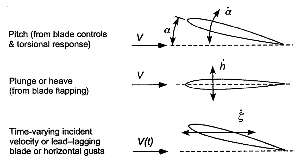
Unsteady airfoil motion components [taken from Principles in Helicopter Aerodynamics by JG Leishman]

The idea with regard to accounting for unsteady aerodynamic effects on rotors is not unlike the steady aerodynamics. The NSE are time dependent so, in principle, solving those equations gives one the aerodynamic forces and moments as a function of time. However, the reason that this is not done is not just that one would have to wait a anywhere from a few hours to a few days for simple simulations. As was stressed in the review chapter on 2D aerodynamics solving the complete set of NSE, while exact, is less amenable to intuitive understanding of the phenomena being modelled. Which is why all the engineering theories that were proposed in an effort to understand fluid behavior on lifting bodies, in the aftermath of the first powered aircraft flight, were all highly intuitive and based on direct verifiable evidence.

Steady airfoil aerodynamics¶

Steady airfoil aerodynamics has already been covered in the ‘Blade Element Theory’ section.

Quasi-steady airfoil aerodynamics¶

Quasi-steady modelling of airfoil aerodynamics leads to a similar result as the steady modelling case provided the effective angle of attack is measured at the three quarter-chord position. While the following result can be derived using concepts already discussed in the review chapter, that is not the subject of this chapter and can be assumed to be agiven.

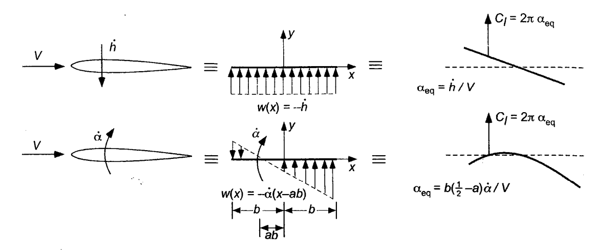
\[C_l = 2\pi\left [\alpha +\frac{\dot{h}}{V}+b \left ( \frac{1}{2}-a \right ) \frac{\dot{\alpha}}{V} \right] = 2\pi\alpha_{3c/4}\]

Quasi-steady airfoil aerodynamics [source])

Unsteady aerodynamics¶

This is the subject of this chapter.

Unsteady airfoil aerodynamics: Overview¶

Whenever a quick change in the flow conditions or the airfoil angle of attack occurs, the airfoil aerodynamics can be very different from its steady/quasi-steady counterpart. That said, the very concepts that help analyse the physics of steady airfoil aerodynamics, and quantify the aerodynamic forces, can be used to explain the physics behind the aerodynamic behavior of unsteady airfoils.

Step change in $\alpha$¶

The figure below shows the build-up of lift when the angle of attack of is changed instantaneously. The airfoil lift coefficient ($C_L$), instead of following an instantaneous change, undergoes a gradual rise in $C_L$ and theoretically reaching the steady state value at infinite time. The peculiar aspect about the form of the $C_L$ curve is that it is no longer directly proportional to $\alpha$, with the proportionality constant given by $2\pi$ from thin airfoil theory. We will later discuss the Theodorsen theory to predict this unsteady behavior of pitching and plunging airfoils with reasonable accuracy. This theory is based on potential flow assumption so clearly this delay in lift exhibited is not somehow related to compressibility of the fluid (incompressiblity assumption used in potential flow analyses).

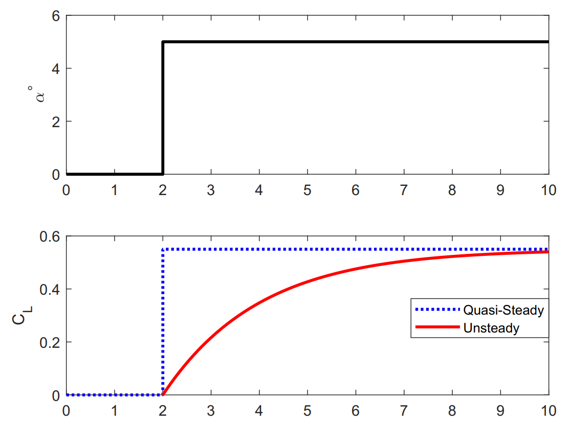
Airfoil lift developement after step-input [source]

The above result is not purely of academic interest. Autogyros1 are capable of undertaking a jump take-off where the rotors are spun to high RPM at zero collective and then a rapid increase in collective allows the autogyro to take off as a helicopter. While the change in blade section $\alpha$ is not exactly instantaneous, the central point is that the associated unsteadiness cannot be ignored if one needs to accurately quantify blade aerodynamic forces. Such unsteady development of aerodynamic forces is also central to understanding what amount of forces are generated, for e.g., on fixed-wing fighter aircraft during a rapid pitch-up manuever. Large civilian fixed-wing aircraft typically never undergo maneuvers rapid enough for unsteady effects to be of any substantial effect, wing flutter phenomenon being the exception, so quasi-steady aerodynamic modelling suffices.

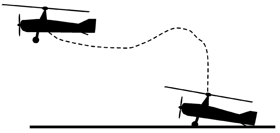
Schematic showing an autogyro undergoing a jump take-off [source]

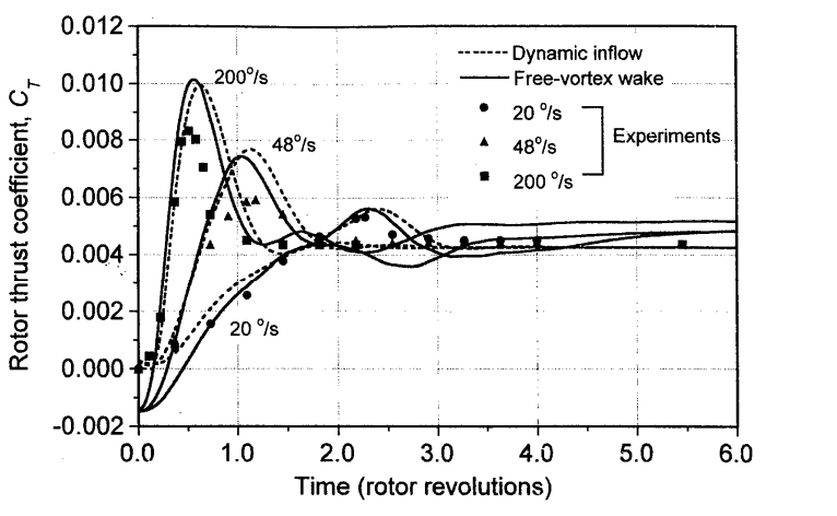
Effect of "ramp" increase in rotor collective on rotor thrust [source])

At first sight the results corresponding to step change in airfoil $\alpha$ and ramp change in rotor collective (which by extension can be seen as a ramp change in blade section $\alpha$) might suggest that there are different aerodynamic mechanisms at play here in the two scenarios. The unsteady lift approaches the steady state lift assymptotically from the bottom while there is a clear overshoot in the latter case. This is in part because the former is a purely 2D case but the latter is a 3D aerodynamics case. From the ensuing discusion it’ll be clear that fundamentally similar aerodynamic phenomena are responsible for responses observed in either cases.

Harmonic change in $\alpha$¶

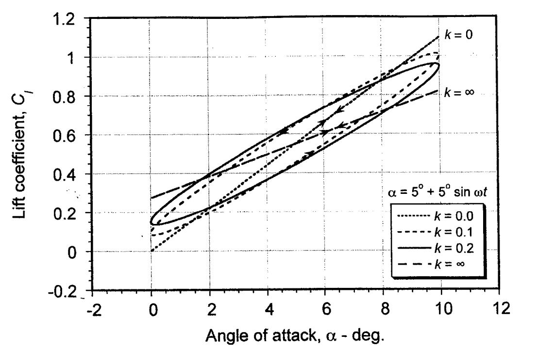
Effect of airfoil pitching motion on aerodynamic lift [taken from Principles in Helicopter Aerodynamics by JG Leishman]

Continuously changing $\alpha$¶

from IPython.display import YouTubeVideo
YouTubeVideo('srjbnvTWRJI', width=800, height=400)

Relevant concepts needed¶

Some of the necessary concepts for steady fluid analysis have already been covered in the review lecture. Here we build on those concepts and extend them to analyse unsteady fluid behavior.

An understanding of the following lies at the heart of developing an intuition for why the unsteady aerodynamics theories were formulated the way they were.

NSE to potential flow theory model
circulatory effect of lifting flow
Kutta-Joukowski theorem
Kelvin’s theorem of circulation
Kutta condition

There are 4 fundamental constructs in potential flow theory that, when used in combination, help fully define potential flow about any body of any given shape [HCCV13](Pg 157). These constructs are parallel uniform flow, sources, sinks, doublets and point vortex. Sources and sinks are essentially the same construct since all that changes between them is the sign of the flow direction. Next we discuss about the final concept that is required before formally looking at the derivation of the Theodorsen unsteady airfoil theory.

Conformal mapping¶

The development of the potential flow theory to analyse flow around a spinning cylinder and the resultant lift have already been discussed. However, one would imagine that being able to carry out the same excercise for an airfoil would be a more fruitful excercise. And you wouldn’t be wrong but the analysis of the flow around a cylinder, albeit seldom relevant for aerospace applications, is directly related to airfoil analysis or analysis around any given random geometry. The mathematical framework that bridges the two comes from complex analysis called conformal mapping. It states that a mapping or complex function $F(\xi)$ can be found that transforms a domain $\xi$ to a domain $z$ and conversely a function $F(z)$ exists that carries out the reverse operation. This means that if we can find such a function that maps a circle to an airfoil then using the same function the entire flowfield around the circle (which we already know) can be mapped to that around an airfoil. So we wouldn’t even explicitly be solving the flow around an airfoil, just get the result for a 2D cylinder and apply the transformation. So far so good, but how does a suitable $F(\xi)$ look like?

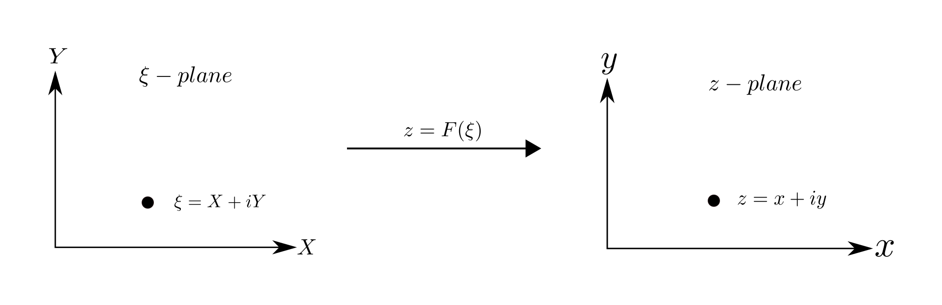
Complex mapping from cylinder domain to airfoil domain

Mapping function¶

Conformal mapping refers to a complex analysis technique of transforming one domain to another while preserving (signed) Euclidean angles. The conformal map that achieves this is called the Joukowski transformation where the body in the $\xi$ domain is a cylinder and it is mapped to a flat plate in the $z$ domain. How exactly the mapping relation itself comes about is a different branch of mathematics altogether but for our purposes suffice it to say that this convenient relation exists and is simple enough to quickly see that indeed the boundary of the circle gets mapped to the boundary of the flat plate.

Before even being able to define $F(\xi)$, what are the properties that $F(\xi)$ should have? For one it needs to be one-to-one i.e. take every point in $\xi$ to a unique point in $z$. In addition, the mapping needs to be differentiable because as we’ll see the velocities get scaled by the derivative at the point of interest. The same is true of the reverse mapping $F(z)$.

\[z = \xi + \frac{a^2}{\xi} \]

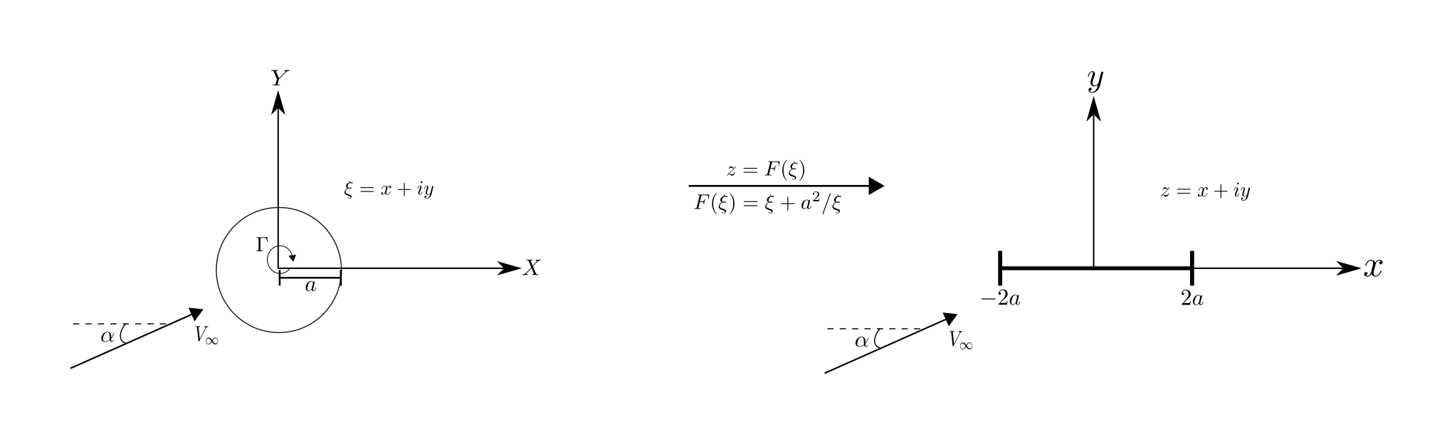
Joukowski transformation from circle to a flat plate (airfoil)

\[\xi = a e^{i\theta}\]

\[\Rightarrow z = \xi + \frac{a^2}{\xi} = 2a\cos \theta\]

The circle in the $\xi$ domain maps to a line of zero thickness in the $z$ domain. This is the airfoil of interest in this case with zero thickness and the leading and trailing edges located at $x = -2a$ and $+2a$, respectively.

Once the mapping function itself is known, it is relatively straightforward to obtain the flowfield around an airfoil once the flowfield around the cylinder is known. Now, it is one thing to obtain the simplest combination of elementary flows that results in a circular streamline (i.e. doublet in uniform flow) and whole different level of complexity to ensure, that given any kind of flow field, i.e. any combination of elementary flows, a circular streamline can be established. For e.g. the solution of the flow field around a circle in uniform flow was already derived but what if the flow now has an ‘angle of attack’ as shown above? This is where the circle theorem proposed by Milne-Thompson [MT40] comes in.

Circle theorem

The circle theorem helps obtain the complex flow field around a cylinder in the most general case. It states that if $F(z)$ is the flow field in the absence of the cylinder then the flow field in the presence of the cylinder is given by $F(z)+\bar{F}(\frac{a^2}{z})$. The solution is based on the idea of images such that a streamline denoting a solid boundary defines a circle. More details can be obtained from [Bat00](Page 422-423) and [MT40].

Using the circle theorem, the flow field around the cylinder without any circulation is given by

\[\begin{equation*} \begin{split} F_{total} &=F(\xi)+\bar{F}(\frac{a^2}{\xi}) \\ &= U_\infty e^{-i\alpha} \xi + \overline{U_\infty e^{-i\alpha} \frac{a^2}{\bar{\xi}}} \\ &=U_\infty e^{-i\alpha} \xi + U_\infty e^{i\alpha} \frac{a^2}{\xi} \end{split} \end{equation*}\]

With the circulation $\Gamma$, the flow field is given by

\[F_{total} = U_\infty e^{-i\alpha} \xi + U_\infty e^{i\alpha} \frac{a^2}{\xi}+ \frac{\Gamma}{2\pi i}\text{ln} \xi \]

Note that we added the potential due to a vortex at the center of the cylinder later since the vortex does not disturb the circular streamline already established by the application of the circle theorem. The velocity field can be obtained both in the $\xi$ domain as well as the $z$ domain. Note that we are primarily interested in the velocity at the surface of the geometry itself because the pressure distribution, and by extension the total lift, can be then obtained using the Bernoulli’s equation.

\[\frac{d F}{d \xi}=U_{\infty} e^{-i \alpha}-U_{\infty} e^{i \alpha} \frac{a^2}{\xi^2}-\frac{\Gamma}{2 \pi i \xi}\]

Velocity at the cylinder surface

\[\Rightarrow w(\xi) = F'(|\xi|=a) = \frac{d F}{d \xi} =U_\infty e^{-i\alpha}-U_\infty e^{i(\alpha-2 \theta)}+\frac{i\Gamma}{2 \pi a} e^{-i \theta}\]

Similarly, velocity in the $z$ domain can be obtained using the complex formula that relates derivatives in the two domains related via a conformal transformation

\[\begin{equation*} \begin{split} w(z)&=\frac{w(\xi)}{\frac{d z}{d\xi}} \\ &=\frac{\frac{d F}{d\xi}}{{1-a^2 / \xi^2}}\\ &=\frac{U_{\infty} e^{-i \alpha} \xi - U_{\infty} e^{i \alpha}\frac{a^2}{\xi}-\frac{\Gamma}{2 \pi i}}{\xi-\frac{a^2}{\xi}}\\ & =\frac{U_{\infty} \cos \alpha \left(\xi-\frac{a^2}{\xi}\right)-i U_{\infty} \sin \alpha \left(\xi+\frac{a^2}{\xi}\right)-\frac{\Gamma}{2 \pi}}{\xi-\frac{a^2}{\xi}} \\ & =U_{\infty} \cos \alpha-i \frac{U_{\infty} z\sin \alpha - \frac{\Gamma}{2 \pi}}{\xi-\frac{a^2}{\xi}} \\ & =U_{\infty} \cos \alpha-i \frac{U_{\infty} z\sin \alpha - \frac{\Gamma}{2 \pi}}{\sqrt{z^2-4a^2}} \\ \end{split} \end{equation*}\]

Kutta condition¶

It was already stated in the context of a cylinder that the lift generated is entirely dependent on the circulation. This is true also in the case of the mapped velocity distribution around the airfoil of zero thickness in the $z$ domain. We call the mapped zero-thickness geometry in the $z$ domain an airfoil because the same circulation $\Gamma$ is also sustained now in the $z$ domain. Recall that $\Gamma$ is an arbitrary quantity but lift generated by an airfoil at a given angle of attack is unique and is directly dictated by the amount of $\Gamma$. So how is a unique $\Gamma$ established at a given angle of attack $\alpha$. This is where the empirically established Kutta condition comes in.

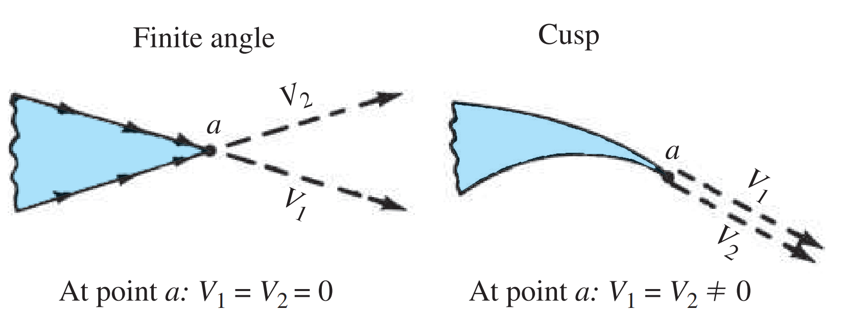
Kutta condition based on the nature of the trailing edge shape. [source]

It is worth noting that the velocity over the airfoil $w(z)$ blows up at $z=\pm 2a$ unless the numerator $U_{\infty} z\sin \alpha - \frac{\Gamma}{2 \pi}$ goes to zero too. Problem is that the denominator goes to zero at $z=\pm 2a$ but the numerator can only be made zero at either the trailing edge $+2a$ or the leading edge $-2a$. The Kutta condition states that the velocity at the trailing edge needs to be finite so the unique circulation then obtained is given by

\[\Gamma = 4 \pi a U_{\infty}\sin \alpha = 2\pi c U_{\infty}\sin \alpha\]

Using the Kutta-Joukowski relation and the definition of coefficient of lift

\[C_L = 2\pi \sin \alpha \approx 2\pi \alpha\]

Using the Bernoulli’s equation, the pressure distribution is given by -

\[p(x) = \rho U_\infty^2\sin 2\alpha \sqrt{\frac{a - x}{a+x}}\]

The center of pressure then turns out to be at the quarter chord. Note that the potential flow theory formulation still leaves the unphysical infinite velocity at the leading edge unresolved. However, this is considered acceptable because in reality a high pressure suction peak is observed at the leading edge but not at the trailing edge. Potential flow solution with the Kutta condition imposed is qualitatively able to reproduce that scenario and the infinite velocity at $z=-2a$ can be considered as a mathematical consequence of idealisation of the flow within the framework of potential flow theory.

Further results/discussion¶

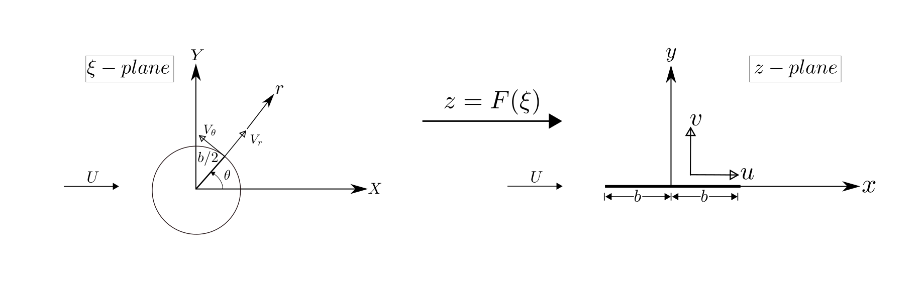
Complex mapping from cylinder to an airfoil

Using the Joukowski’s conformal mapping, the surface of a cylinder maps to a flat plate along the x-axis.

\[ r=\frac{1}{2} b \longrightarrow -b \leq x \leq b, \quad y=0 \]

Each point (X,Y) maps to (x,y) according to the following relations-

\[z = \xi + \frac{b^2}{4\xi} \]

\[\Rightarrow x+i y=(X+i Y)+\frac{b^2}{4(X+i Y)}\]

\[\begin{split} \begin{gathered} X=r \cos \theta, \quad Y=r \sin \theta, \\ X+i Y=r(\cos \theta+i \sin \theta)=r e^{i \theta} \end{gathered} \end{split}\]

\[x=b \cos \theta, \quad y=0 \]

Similarly, position on the X-axis transform in the z-domain to the x-axis.

\[ x=X+b^2 / 4 X, \quad y=Y=0 \]

The velocities between the two domains get mapped as shown below.

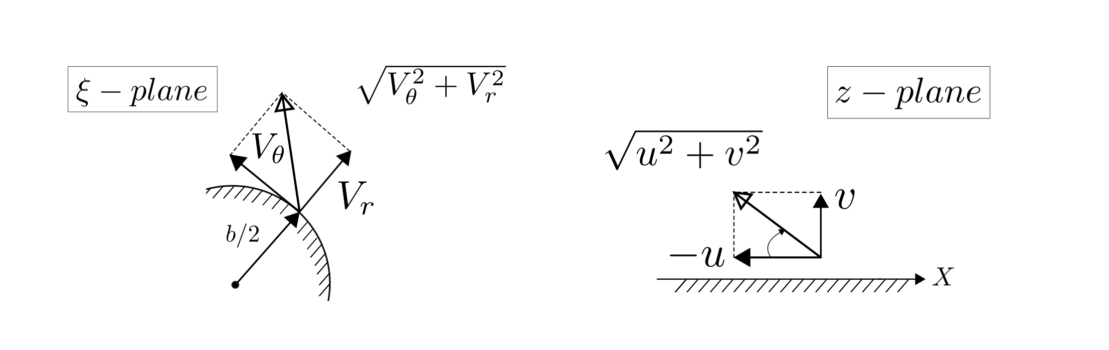
Velocity transformation from the $\xi$-domain to the $z$-domain

\[ u-i v=\frac{V_X-i V_Y}{[d(x+i y) / d(X+i Y)]} \]

\[\begin{split} \begin{aligned} {\left[\frac{d(x+i y)}{d(X+i Y)}\right]_{r = b / 2} } & =\left[1-\frac{b^2}{4(X+i Y)^2}\right]_{r=b / 2} \\ & =1-\frac{b^2}{b^2 e^{i 2 \theta}}=2 \sin \theta e^{i \theta} \end{aligned} \end{split}\]

\[\left|u-i v\right|=\sqrt{u^2+v^2}=\frac{\sqrt{V_X^2+V_Y^2}}{|2 \sin \theta|}=\frac{\sqrt{V_\theta^2+V_r^2}}{|2 \sin \theta|}\]

Therefore the flow velocities in the two domains are related as-

\[\begin{split} \begin{aligned} & \left|u\right|=\frac{\left|V_\theta\right|}{|2 \sin \theta|}, \\ & |v|=\frac{\left|V_r\right|}{|2 \sin \theta|} \end{aligned} \end{split}\]

And in the domain $0 \leq \theta \leq \pi$, for e.g.,

\[\begin{split} \left.\begin{array}{l} V_\theta=-2 u \sin \theta \\ V_r=2 v \sin \theta, \end{array}\right\} 0 \leq \theta \leq \pi \end{split}\]

Note

If the tangential flow velocity at in the cylinder domain is non-zero at $\theta=0$ then that translates to $u=\infty$ at the trailing-edge of the airfoil in the z-domain.

Based on the velocity distribution, the corresponding potential function on the airfoil surface $\phi(x)$ can be obtained-

\[\phi(x_1)-\phi(x_2) = \int_{x_2}^{x_1}\frac{\partial \phi}{\partial x} dx\]

and in particular

\[\phi(x)-\phi_{LE} = \int_{LE}^{x}\frac{\partial \phi}{\partial x} dx\]

Additionally, unlike the stream function $\psi$, the value of the scalar potential function $\phi$ itself at a given point does not have a physical meaning. It is the derivatives of $\phi$ that need to satisfy the relevant conditions so the value at any given location can be chosen as the reference and set to 0. In this case $\phi_{LE}=0$ is assumed to simplify the above expression. Also, to avoid confusion the variable of integration is changed to $\varphi$ in order to use the polar coordinates instead of Cartesian coordinates.

\[\begin{equation*} \begin{split} \phi(\theta) &= \int_{\pi}^{\theta}\frac{-V_\theta}{2\sin \varphi} (-b\sin \varphi d\varphi) \\ &=\frac{-b}{2}\int_{\theta}^{\pi}V_\theta d\varphi \end{split} \end{equation*}\]

So once the tangential flow velocity around a cylinder is known, the potential function can be obtained in a straightforward manner.

Linearised unsteady Bernoulli’s equation¶

The general unsteady Bernoulli’s equation is given by the following expression

\[\frac{\partial \phi}{\partial t}+\frac{|\nabla \phi|^2}{2}+F+\frac{p}{\rho}=\text { constant }\]

Where, $\left | F \right |=gz$ is the body force acting on the fluid and can be neglected for our purposes since the fluid flows horizontally. Assume the above expression to be given (for derivation one can consult Section 2.12 in [Sen14]).

\[\begin{equation*} \begin{split} p-p_\infty = & -\rho\left [ \frac{\partial \phi}{\partial t}+\frac{|\nabla \phi|^2-U_\infty^2}{2} \right ] \\ & = -\rho\left [ \frac{\partial \phi}{\partial t}+\frac{|\mathbf{V}|^2-U_\infty^2}{2} \right ] \\ & \approx -\rho\left [ \frac{\partial \phi}{\partial t}+U_\infty u \right ] \\ & = -\rho\left [ \frac{\partial \phi}{\partial t}+U_\infty \frac{\partial \phi}{\partial x} \right ] \end{split} \end{equation*}\]

Here $|\nabla \phi|^2 = |\mathbf{V}|^2$ is a non-linear term which has been linearised about the mean flow velocity of $U_\infty$. Additionally, $\mathbf{V} = (u+U_\infty)\hat{i}+v\hat{j}$ was assumed in the above derivation where $u$ and $v<<U_\infty$.

So once the potential function on the surface of the airfoil is known, the total unsteady lift at a given instant of time can be evaluated in a straightforward manner.

Unsteady Development of Steady lift¶

We now know that in case of an impulsively started flow, Kelvin’s theorem needs to apply and consequently a starting vortex is shed in the wake as a vorticity of equal magnitude develops around the airfoil. In reality, this circulation develops due to the viscous property of fluids which is completely ignored in the potential flow theory that has been used as the modelling strategy. Instead, the Kutta condition has been used to uniquely quantify the circulatory effect around the airfoil. Based on the level of modelling fidelity, the total lift can be evaluated either assuming distributed vorticity or concentrated vorticity.

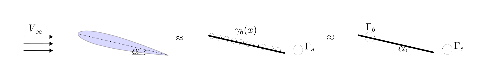
Two levels of modelling instantaneous circulation due to bound and starting vortex after impulsive start of flow

Since the starting vortex is close to the airfoil it induces a velocity on the surface of the airfoil much like the induced velocity concept we’ve now become familiar with in the context of finite-wing theory. So even 2D airfoils experience an induced velocity when unsteadiness is accounted for, steady airfoils don’t!. As time progresses the starting vortex drifts away from the airfoil and the corresponding induced velocity effect on the airfoil decreases. After sufficiently long time, the effect of the starting vortex is negligible such that even its mere presence is ignored and we have the familiar picture of steady-state lift generation around an airfoil represented as bound vorticity that we are familiar with.

Two levels of modelling instantaneous circulation due to bound and starting vortex after impulsive start of flow

Unsteady Lift due to Airfoil Motion¶

Now, extending the above strategy of modelling unsteadiness when the airfoil is undergoing motion such that its angle of attack is constantly changing. Using the physical model that has been used until now based on established fluid dynamics prinicples, airfoil motion immediately implies changing angle of attack. This in turn means a varying bound circulation around the airfoil and, therefore, more ‘starting’ vortices except now they are refered to as shed vortices. Like the starting vortex, shed vortices are emanated from the airfoil trailing-edge and thereafter move with the free stream and their effect on the airfoil can be neglected when they get far from the airfoil. However, due to the varying bound vorticity around the airfoil there is new shed vortices continuously introduced into the flow from the trailing-edge. Even after sufficiently long time the lift generated by the airfoil will not reach a steady state because - 1) the airfoil is moving so the angle of attack is not constant and 2) the airfoil is continuously under the influence of induced velocity of shed vortices. The shed vortices are continuously drifting away from the airfoil so their effect on the airfoil is also continuously varying. Keeping track of this time varying strength and position of shed vortices, in order to quantify their influence on the airfoil, and thereby help evaluate the net lift generated by the airfoil, is what unsteady aerodynamics analysis is all about in a nutshell. If you do not account for the effect of the wake, then one ends up with the steady aerodynamics domain of analysis.

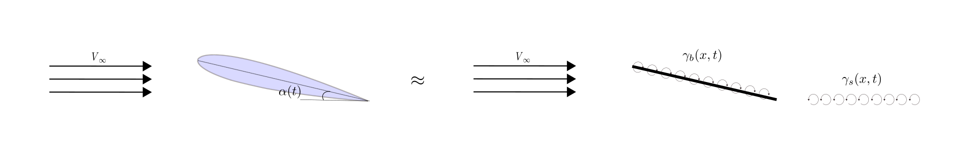
Instantaneous circulation due to bound and starting vortex after impulsive start of flow

Next we look at the classical Theordorsen model to predict unsteady pressure distribution around thin airfoils.

1: They are a class of rotorcraft where an unpowered rotor spins in windmill operating state during flight to generate the vertical thrust necessary to stay aloft while a propeller generates horizontal thrust to overcome drag from the free-spinning rotor. On some designs a clutch mechanism allows to divert engine power to the rotor for initial spin-up while on the ground to facilitate the jump take-off maneuver.

Recap of Fundamentals in Aerodynamics - 2D and 3D

Theodorsen Theory

Fundamentals of Helicopter Aerodynamics